3. The Jupyter notebook cheat sheet

This document will be available to you during tests and exams

3.1. Table of Contents

Numeric

Basic plotting functions

Symbolic manipulation

Equation solving

Matrix math

import tbcontrol
tbcontrol.expectversion('0.1.2')

3.2. Numeric

import numpy
import scipy

a = numpy.array([1, 2, 3])

t = numpy.linspace(0, 10)

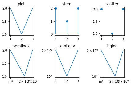
3.3. Basic plotting functions

import matplotlib.pyplot as plt
%matplotlib inline

plotfuncs = [plt.plot,
             plt.stem,
             plt.scatter,
             plt.semilogx,
             plt.semilogy,
             plt.loglog]

for i, func in enumerate(plotfuncs, 1):
    plt.subplot(2, 3, i)
    func([1, 2, 3], [2, 1, 2])
    plt.title(func.__name__)
plt.tight_layout()

3.4. Symbolic manipulation

3.4.1. Imports

import sympy
sympy.init_printing()

Symbol definitions

s = sympy.Symbol('s')  # A single symbol
tau, K_c = sympy.symbols('tau K_c', positive=True) # we can use real=True or complex=True for other kinds of variables

Example controller and system

Gc = K_c*((tau*s + 1) / (tau*s))
GvGpGm = 5 / ((10*s + 1)**2)

3.4.2. Working with rational functions and polynomials

We often want nice rational functions, but sympy doesn’t make expressions rational by default

chareq = GvGpGm*Gc + 1
chareq

$$\frac{5 K_{c} \left(s \tau + 1\right)}{s \tau \left(10 s + 1\right)^{2}} + 1$$

The cancel function forces this to be a fraction. collect collects terms.

chareq = chareq.cancel().collect(s)
chareq

$$\frac{5 K_{c} + 100 s^{3} \tau + 20 s^{2} \tau + s \left(5 K_{c} \tau + \tau\right)}{100 s^{3} \tau + 20 s^{2} \tau + s \tau}$$

In some cases we can factor equations:

chareq.factor(s)

$$\frac{5 K_{c} + 100 s^{3} \tau + 20 s^{2} \tau + s \left(5 K_{c} \tau + \tau\right)}{s \tau \left(10 s + 1\right)^{2}}$$

Obtain the numerator and denominator:

sympy.numer(chareq), sympy.denom(chareq)

$$\left ( 5 K_{c} + 100 s^{3} \tau + 20 s^{2} \tau + s \left(5 K_{c} \tau + \tau\right), \quad 100 s^{3} \tau + 20 s^{2} \tau + s \tau\right )$$

If you want them both, you can use

chareq.as_numer_denom()

$$\left ( 5 K_{c} + 100 s^{3} \tau + 20 s^{2} \tau + s \left(5 K_{c} \tau + \tau\right), \quad 100 s^{3} \tau + 20 s^{2} \tau + s \tau\right )$$

Convert to polynomial in s

numer = sympy.poly(sympy.numer(chareq), s)

Once we have a polynomial, it is easy to obtain coefficients:

numer.all_coeffs()

$$\left [ 100 \tau, \quad 20 \tau, \quad 5 K_{c} \tau + \tau, \quad 5 K_{c}\right ]$$

Calculate the Routh Array

from tbcontrol.symbolic import routh

routh(numer)

$$\left[\begin{matrix}100 \tau & 5 K_{c} \tau + \tau\\20 \tau & 5 K_{c}\\- 25 K_{c} + \tau \left(5 K_{c} + 1\right) & 0\\5 K_{c} & 0\end{matrix}\right]$$

To get a function which can be used numerically, use lambdify:

f = sympy.lambdify((K_c, tau), K_c + tau)

f(1, 2)

$$3$$

3.4.3. Functions useful for discrete systems

z, q = sympy.symbols('z, q')

Gz = z**-1/(1 - z**-1)
Gz

$$\frac{1}{z \left(1 - \frac{1}{z}\right)}$$

Write in terms of positive powers of \(z\):

Gz.cancel()

$$\frac{1}{z - 1}$$

Write in terms of negative powers of \(z\):

Gz.subs({z: q**-1}).cancel()

$$- \frac{q}{q - 1}$$

Inversion of the \(z\) transform

from tbcontrol.symbolic import sampledvalues

sampledvalues(Gz, z, 10)

$$\left [ 0, \quad 1, \quad 1, \quad 1, \quad 1, \quad 1, \quad 1, \quad 1, \quad 1, \quad 1\right ]$$

3.5. Equation solving

3.5.1. Symbolic

x, y, z, a = sympy.symbols('x, y, z, a')
residuals = [x + y - 2, y + z - a, x + y + z]
unknowns = [x, y, z]
sympy.solve(residuals, unknowns)

$$\left \{ x : - a, \quad y : a + 2, \quad z : -2\right \}$$

3.5.2. Numeric sympy

residuals = [2*x**2 - 2*y**2, sympy.sin(x) + sympy.log(y)]
unknowns = [x, y]
sympy.nsolve(residuals, unknowns, [1, 3])

$$\left[\begin{matrix}-2.21910714891375\\2.21910714891375\end{matrix}\right]$$

3.5.3. Numeric

import scipy.optimize

def residuals(unknowns):
    x, y = unknowns
    return [2*x**2 - 2*y**2, numpy.sin(x) + numpy.log(y)]

starting_point = [1, 3]

residuals(starting_point)

$$\left [ -16, \quad 1.9400832734760063\right ]$$

scipy.optimize.fsolve(residuals, starting_point)

array([-2.21910715,  2.21910715])

3.6. Matrix math

3.6.1. Symbolic

G11, G12, G21, G22 = sympy.symbols('G11, G12, G21, G22')

Creation

G = sympy.Matrix([[G11, G12], [G21, G22]])
G

$$\left[\begin{matrix}G_{11} & G_{12}\\G_{21} & G_{22}\end{matrix}\right]$$

Determinant, inverse, transpose

G.det(), G.inv(), G.T

$$\left ( G_{11} G_{22} - G_{12} G_{21}, \quad \left[\begin{matrix}\frac{G_{22}}{G_{11} G_{22} - G_{12} G_{21}} & - \frac{G_{12}}{G_{11} G_{22} - G_{12} G_{21}}\\- \frac{G_{21}}{G_{11} G_{22} - G_{12} G_{21}} & \frac{G_{11}}{G_{11} G_{22} - G_{12} G_{21}}\end{matrix}\right], \quad \left[\begin{matrix}G_{11} & G_{21}\\G_{12} & G_{22}\end{matrix}\right]\right )$$

Math operations: Multiplication, addition, elementwise multiplication:

G*G, G+G, G.multiply_elementwise(G)

$$\left ( \left[\begin{matrix}G_{11}^{2} + G_{12} G_{21} & G_{11} G_{12} + G_{12} G_{22}\\G_{11} G_{21} + G_{21} G_{22} & G_{12} G_{21} + G_{22}^{2}\end{matrix}\right], \quad \left[\begin{matrix}2 G_{11} & 2 G_{12}\\2 G_{21} & 2 G_{22}\end{matrix}\right], \quad \left[\begin{matrix}G_{11}^{2} & G_{12}^{2}\\G_{21}^{2} & G_{22}^{2}\end{matrix}\right]\right )$$

3.6.2. Numeric

Creation

G = numpy.matrix([[1, 2], [3, 4]])

Determinant, inverse, transpose

numpy.linalg.det(G), G.I, G.T

(-2.0000000000000004, matrix([[-2. ,  1. ],
         [ 1.5, -0.5]]), matrix([[1, 3],
         [2, 4]]))

Math operations: Multiplication, addition, elementwise multiplication:

G*G, G+G, G.A*G.A

(matrix([[ 7, 10],
         [15, 22]]), matrix([[2, 4],
         [6, 8]]), array([[ 1,  4],
        [ 9, 16]]))