2. PID step responses

Here are some open loop step responses of PID controllers in different configurations.

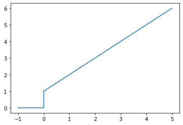
2.1. PI

import control
import numpy
import matplotlib.pyplot as plt
%matplotlib inline

s = control.tf([1, 0], 1)
ts = numpy.linspace(0, 5)

def plot_step_response(G):
    t, y = control.step_response(G, ts)
    # Add some action before time zero so that the initial step is visible
    t = numpy.concatenate([[-1, 0], t])
    y = numpy.concatenate([[0, 0], y])
    plt.plot(t, y)

K_C = 1

tau_I = 1

Gc = K_C*(1 + 1/(tau_I*s))

plot_step_response(Gc)

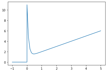
2.2. PID

Because the ideal PID is unrealisable, we can’t plot the response of the ideal PID, but we can do it for the realisable ISA PID.

\[G_c = K_C\left( 1 + \frac{1}{\tau_I s} + \frac{\tau_D s}{\alpha \tau_D s + 1} \right)\]

alpha = 0.1
tau_D = 1

Gc = K_C*(1 + 1/(tau_I*s) + 1*s/(alpha*tau_D*s + 1))

plot_step_response(Gc)

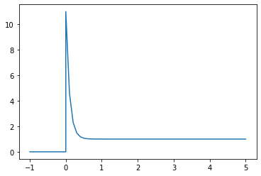
2.3. PD

Gc = K_C*(1 + 1*s/(alpha*tau_D*s + 1))

plot_step_response(Gc)