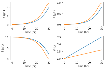
4. Fed Batch Bioreactor

This model represents the fed batch bioreactor in section 2.4.9 of Seborg et al.

Nr	Symbol	Name	Units
1	\(\mu_\text{max}\)	Maximum specific growth rate	1/hr
2	\(K_s\)	Monod constant	g/L
3	\(Y_{X/S}\)	Cell yield coefficient	1
4	\(Y_{P/S}\)	Product yield coefficient	1
5	\(X\)	Cell mass concentration	g/L
6	\(S\)	Substrate mass concentration	g/L
7	\(V\)	Volume	L
8	\(P\)	Substrate mass concentration	g/L
9	\(F\)	Feed flow rate	L/hr
10	\(S_f\)	Substrate mass concentration	g/L
11	\(\mu\)	Specific growth rate	1/hr
12	\(r_g\)	Cell growth rate	g /( L hr)
13	\(r_p\)	Product growth rate	g /( L hr)

Model equations:

Nr	Equation	Inputs	Outputs	Parameters
1	\[r_g = \mu X\]		\(r\), \(\mu\), \(X\)
2	\[\mu = \mu_{max} \frac{S}{K_S + S}\]		\(S\)	\(\mu_\text{max}\), \(K_s\)
3	\[r_p = Y_{P/X}r_G\]		\(r_p\)	\(Y_{P/X}\)
4	\[\frac{d(XV)}{dt} = Vr_g\]		\(V\)
5	\[\frac{d(PV)}{dt} = Vr_p\]		\(P\)
6	\[\frac{d(SV)}{dt} = FS_f - Vr\]	\(F\), \(S_f\)		\(Y_{X/S}\)
7	\[\frac{dV}{dt} = F\]
Number	7	2	7	4

Parameters

mu_max = 0.2  # Maximum growth rate
K_s = 1.0  # Monod constant
Y_xs = 0.5 # Cell yield coefficient
Y_px = 0.2  # Product yield coefficient

States

X = 0.05  # Concentration of the cells
S = 10   # Concentration of the substrate
P = 0   # Concentration of the product
V = 1   # Reactor volume

x0 = [X, S, P, V]  # State vector

Inputs

F = 0.05  # Feed rate
S_f = 10  # Concentration of substrate in feed

def dxdt(t, x):
    [X, S, P, V] = x

    mu = mu_max * S / (K_s + S)
    rg = mu * X
    rp = Y_px * rg
    dVdt = F
    dXdt = 1/V*(V * rg - dVdt*X)
    dPdt = 1/V*(V * rp - dVdt*P)
    dSdt = 1/V*(F * S_f - 1 / Y_xs * V * rg - dVdt*S)

    return [dXdt, dSdt, dPdt, dVdt]

import scipy.integrate
import numpy

import matplotlib.pyplot as plt
%matplotlib inline

tspan = [0, 30]

tsmooth = numpy.linspace(0, 30)

Fs = [0.05, 0.02]

results = []

for F in Fs:
    out = scipy.integrate.solve_ivp(dxdt, tspan, x0, t_eval=tsmooth)
    results.append(out)

names = ['X', 'S', 'P', 'V']
units = {'X': 'g/L', 'S': 'g/L', 'P': 'g/L', 'V': 'L'}

ax = {}

fig, [[ax['X'], ax['P']], [ax['S'], ax['V']]] = plt.subplots(2, 2)

for F, out in zip(Fs, results):
    var = {name: y for name, y in zip(names, out.y)}
    for name in names:
        ax[name].plot(out.t, var[name])
        ax[name].set_ylabel(f'{name} ({units[name]})')
        ax[name].set_xlabel('Time (hr)')
plt.tight_layout()