3. Laplace transforms in SymPy

The Laplace transform is

\[\mathcal{L}\{f(t)\} = \int_0^\infty f(t) e^{-st} \mathrm{d}s\]

import sympy
sympy.init_printing()

import matplotlib.pyplot as plt
%matplotlib inline

Let’s define some symbols to work with.

t, s = sympy.symbols('t, s')
a = sympy.symbols('a', real=True, positive=True)

3.1. Direct evaluation

We start with a simple function

f = sympy.exp(-a*t)
f

$\displaystyle e^{- a t}$

We can evaluate the integral directly using integrate:

sympy.integrate(f*sympy.exp(-s*t), (t, 0, sympy.oo))

$\displaystyle \begin{cases} \frac{1}{s \left(\frac{a}{s} + 1\right)} & \text{for}\: \left|{\arg{\left(s \right)}}\right| \leq \frac{\pi}{2} \\\int\limits_{0}^{\infty} e^{- a t} e^{- s t}\, dt & \text{otherwise} \end{cases}$

3.2. Library function

This works, but it is a bit cumbersome to have all the extra stuff in there.

Sympy provides a function called laplace_transform which does this more efficiently. By default it will return conditions of convergence as well (recall this is an improper integral, with an infinite bound, so it will not always converge).

sympy.laplace_transform(f, t, s)

$\displaystyle \left( \frac{1}{a + s}, \ - a, \ \text{True}\right)$

If we want just the function, we can specify noconds=True.

F = sympy.laplace_transform(f, t, s, noconds=True)
F

$\displaystyle \frac{1}{a + s}$

We will find it useful to define a quicker version of this:

def L(f):
    return sympy.laplace_transform(f, t, s, noconds=True)

Inverses are simple as well,

def invL(F):
    return sympy.inverse_laplace_transform(F, s, t)

invL(F)

$\displaystyle e^{- a t} \theta\left(t\right)$

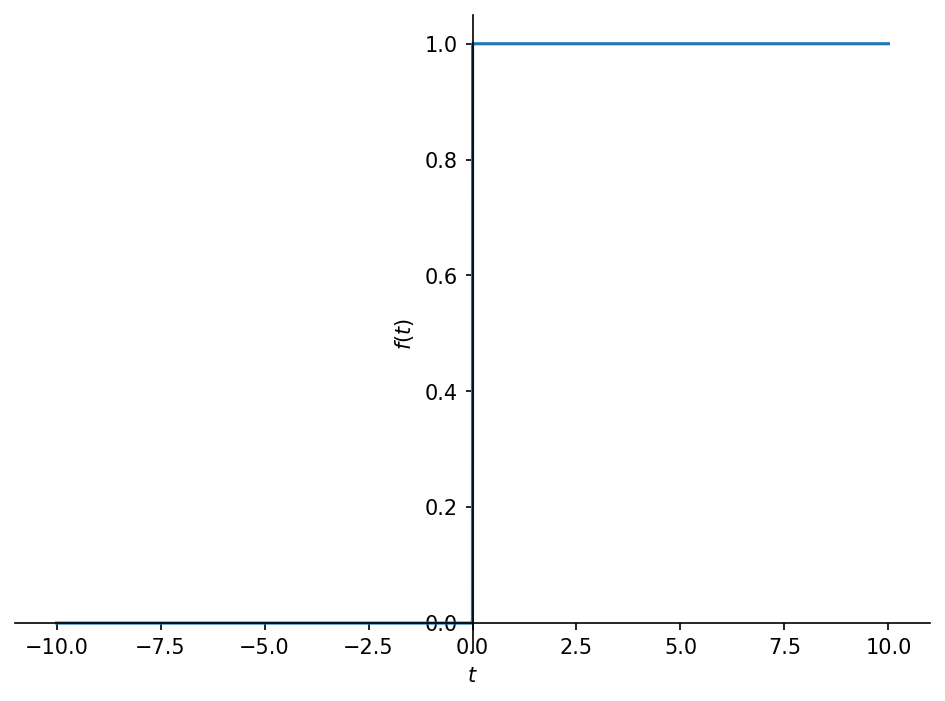
3.3. What is that θ?

The unit step function is also known as the Heaviside step function. We will see this function often in inverse laplace transforms. It is typeset as \(\theta(t)\) by sympy.

sympy.Heaviside(t)

$\displaystyle \theta\left(t\right)$

sympy.plot(sympy.Heaviside(t));

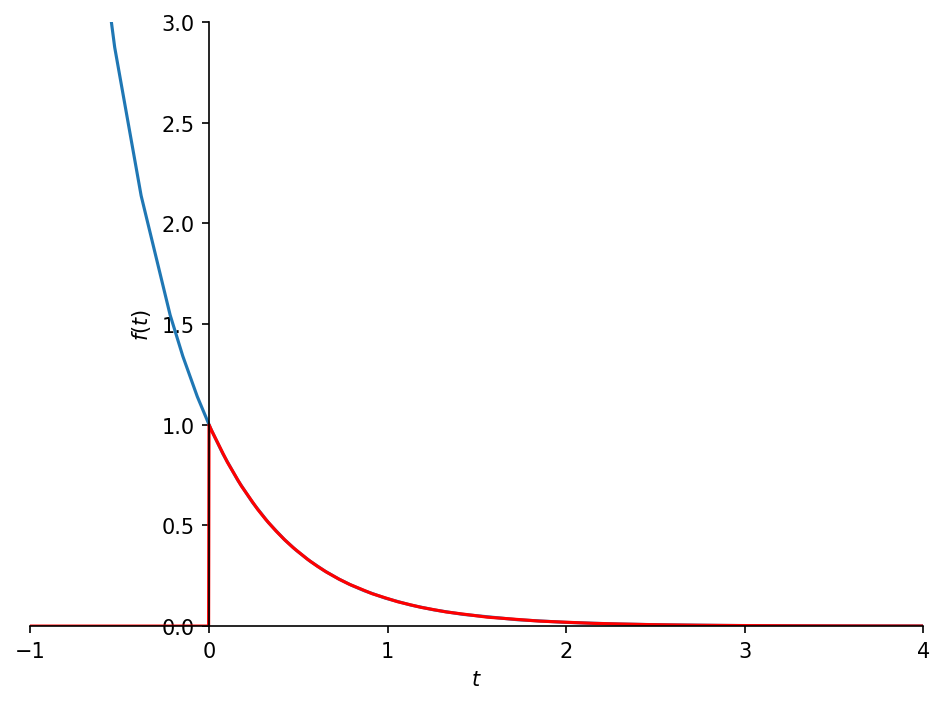
Look at the difference between \(f\) and the inverse laplace transform we obtained, which contains the unit step to force it to zero before \(t=0\).

invL(F).subs({a: 2})

$\displaystyle e^{- 2 t} \theta\left(t\right)$

p = sympy.plot(f.subs({a: 2}), invL(F).subs({a: 2}),
               xlim=(-1, 4), ylim=(0, 3), show=False)
p[1].line_color = 'red'
p.show()

3.4. Reproducing standard transform table

Let’s see if we can match the functions in the table

omega = sympy.Symbol('omega', real=True)
exp = sympy.exp
sin = sympy.sin
cos = sympy.cos
functions = [1,
         t,
         exp(-a*t),
         t*exp(-a*t),
         t**2*exp(-a*t),
         sin(omega*t),
         cos(omega*t),
         1 - exp(-a*t),
         exp(-a*t)*sin(omega*t),
         exp(-a*t)*cos(omega*t),
         ]
functions

$\displaystyle \left[ 1, \ t, \ e^{- a t}, \ t e^{- a t}, \ t^{2} e^{- a t}, \ \sin{\left(\omega t \right)}, \ \cos{\left(\omega t \right)}, \ 1 - e^{- a t}, \ e^{- a t} \sin{\left(\omega t \right)}, \ e^{- a t} \cos{\left(\omega t \right)}\right]$

Fs = [L(f) for f in functions]
Fs

$\displaystyle \left[ \frac{1}{s}, \ \frac{1}{s^{2}}, \ \frac{1}{a + s}, \ \frac{1}{\left(a + s\right)^{2}}, \ \frac{2}{\left(a + s\right)^{3}}, \ \frac{\omega}{\omega^{2} + s^{2}}, \ \frac{s}{\omega^{2} + s^{2}}, \ - \frac{1}{a + s} + \frac{1}{s}, \ \frac{\omega}{\omega^{2} + \left(a + s\right)^{2}}, \ \frac{a + s}{\omega^{2} + \left(a + s\right)^{2}}\right]$

We can make a pretty good approximation of the table with a little help from pandas

from pandas import DataFrame

def makelatex(args):
    return ["$${}$$".format(sympy.latex(a)) for a in args]

DataFrame(list(zip(makelatex(functions), makelatex(Fs))))

	0	1
0	$$1$$	$$\frac{1}{s}$$
1	$$t$$	$$\frac{1}{s^{2}}$$
2	$$e^{- a t}$$	$$\frac{1}{a + s}$$
3	$$t e^{- a t}$$	$$\frac{1}{\left(a + s\right)^{2}}$$
4	$$t^{2} e^{- a t}$$	$$\frac{2}{\left(a + s\right)^{3}}$$
5	$$\sin{\left(\omega t \right)}$$	$$\frac{\omega}{\omega^{2} + s^{2}}$$
6	$$\cos{\left(\omega t \right)}$$	$$\frac{s}{\omega^{2} + s^{2}}$$
7	$$1 - e^{- a t}$$	$$- \frac{1}{a + s} + \frac{1}{s}$$
8	$$e^{- a t} \sin{\left(\omega t \right)}$$	$$\frac{\omega}{\omega^{2} + \left(a + s\right...
9	$$e^{- a t} \cos{\left(\omega t \right)}$$	$$\frac{a + s}{\omega^{2} + \left(a + s\right)...

3.5. More complicated inverses

Why doesn’t the table feature more complicated functions? Because higher-order rational functions can be written as sums of simpler ones through application of partial fractions expansion.

F = ((s + 1)*(s + 2)* (s + 3))/((s + 4)*(s + 5)*(s + 6))

F

$\displaystyle \frac{\left(s + 1\right) \left(s + 2\right) \left(s + 3\right)}{\left(s + 4\right) \left(s + 5\right) \left(s + 6\right)}$

F.apart(s)

$\displaystyle 1 - \frac{30}{s + 6} + \frac{24}{s + 5} - \frac{3}{s + 4}$

In most cases, sympy will be able to figure out how to do the right thing with most of the functions we use, even the hard ones. Notice the relationship between this inverse Laplace and the expression we obtained above:

invL(F)

$\displaystyle \delta\left(t\right) - 3 e^{- 4 t} \theta\left(t\right) + 24 e^{- 5 t} \theta\left(t\right) - 30 e^{- 6 t} \theta\left(t\right)$