import numpy
import matplotlib.pyplot as plt
%matplotlib inline

3. Read simulation input from a file

It is often useful to read simulation inputs from a file. Let’s do this for our standard tank system.

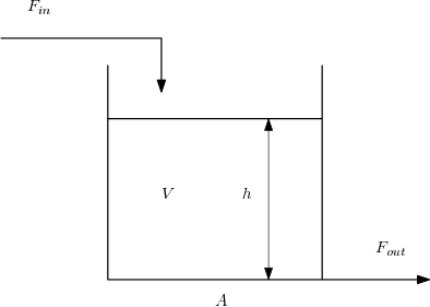
\begin{align} F_{out} &= kh\\ \frac{\mathrm{d}h}{\mathrm{d}t} &= \frac{1}{A}\left(F_{in} - F_{out}\right)\\ \end{align}

First we define the parameters of the system

K = 1
A = 1

Then, we’ll read the values of \(F_{in}\) from an Excel file using pandas.read_excel.

import pandas

df = pandas.read_excel('../../assets/tankdata.xlsx')
df

	Time	Fin
0	0	1.0
1	5	2.0
2	10	2.0
3	15	1.5
4	20	1.0
5	25	2.0
6	30	2.0

We’ll set this function up to interpolate on the above table for the value of \(F_in\) given a known time.

def Fin(t):
    return numpy.interp(t, df.Time, df.Fin)

We can test for one value at a time

Fin(1)

1.2

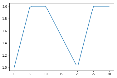
interp also accepts vector inputs:

tspan = (0, 30)
t = numpy.linspace(*tspan)

plt.plot(t, Fin(t))

[<matplotlib.lines.Line2D at 0x112b4c208>]

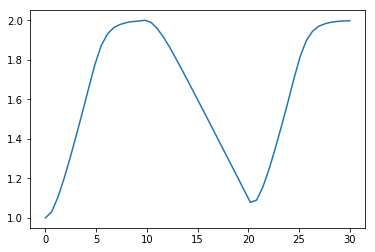
Now we’re ready to define our differential equation function:

def dhdt(t, h):
    Fout = K*h
    return 1/A*(Fin(t) - Fout)

h0 = 1

import scipy.integrate

sol = scipy.integrate.solve_ivp(dhdt, tspan, [h0], t_eval=t)

plt.plot(sol.t, sol.y.T)

[<matplotlib.lines.Line2D at 0x1513ee6b38>]