[1]:

import matplotlib.pyplot as plt
%matplotlib inline

[2]:

import numpy

[3]:

from tbcontrol import blocksim

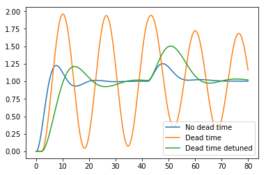
1. Dead time reduces control performance

Let’s first build a standard control loop with a disturbance.

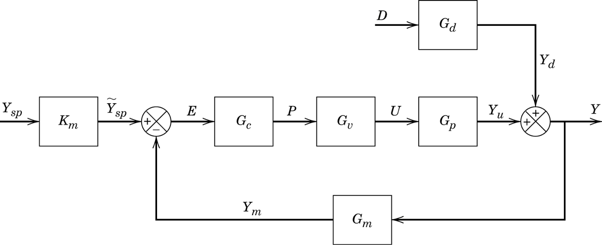
42c46a774442485fafe162afe5b30641

We’ll use the system and simulate the control performance with and without deadtime. \(K_m=G_c=G_m=1\) and

\[G_p = G_d = \frac{e^{-\theta s}}{(5s + 1)(3s + 1)}\]

[4]:

inputs = {'ysp': blocksim.step(),
          'd': blocksim.step(starttime=40)}

[5]:

sums = {'y': ('+yu', '+yd'),
        'e': ('+ysp', '-y'),
        }

For the dead time free system, we can use a high gain PI controller

[6]:

def Gp(name, input, output, theta):
    return blocksim.LTI(name, input, output,
                        1, numpy.convolve([5, 1], [3, 1]), delay=theta)

[7]:

Gp1 = Gp('Gp', 'p', 'yu', 0)

[8]:

Gc1 = blocksim.PI('Gc', 'e', 'p',
                  3.02, 6.5)

For the system with dead time we need to detune the controller

[9]:

Gp2 = Gp('Gp', 'p', 'yu', 2)

[10]:

Gc2 = blocksim.PI('Gc', 'e', 'p',
                  1.23, 7)

[11]:

Gd = Gp('Gd', 'd', 'yd', 2)

[12]:

diagrams = {'No dead time': blocksim.Diagram([Gp1, Gc1, Gd], sums, inputs),
            'Dead time': blocksim.Diagram([Gp2, Gc1, Gd], sums, inputs),
            'Dead time detuned': blocksim.Diagram([Gp2, Gc2, Gd], sums, inputs)
           }

[13]:

ts = numpy.linspace(0, 80, 2000)

[14]:

outputs = {}

[15]:

for description, diagram in diagrams.items():
    lastoutput = outputs[description] = diagram.simulate(ts)
    plt.plot(ts, lastoutput['y'], label=description)
plt.legend()

[15]:

<matplotlib.legend.Legend at 0x1c1f7ade10>

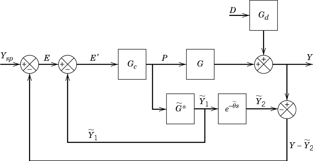
../../_images/2_Control_5_Advanced_control_methods_Dead_time_compensation_19_1.png

2. Smith Predictor

The Smith predictor or dead time compensator uses a dead time free model to do most of the control (\(\widetilde{G}^*\)} and then subtracts the delayed prediction from the measurement to react only on the unhandled dynamics.

2f9c7b5a1cd84fa6a495101bdd3254ae

[16]:

sums = {'y': ('+yd', '+yu'),
        'y-ytilde2': ('-ytilde2', '+y'),
        'e': ('+ysp', '-y-ytilde2'),
        'eprime': ('+e', '-ytilde1'),
       }

We’ll use the dead time containing model from before

[17]:

G = Gp2
G.name = 'G'

But the controller which was tuned on the dead time free model

[18]:

Gc = Gc1
Gc.inputname = 'eprime'

[19]:

Gtildestar = blocksim.LTI('Gtildestar', 'p', 'ytilde1',
                          1, numpy.convolve([5, 1], [3, 1]))

[20]:

delay = blocksim.Deadtime('Delay', 'ytilde1', 'ytilde2', 2)

[21]:

blocks = [Gc, G, Gd, Gtildestar, delay]

[22]:

diagram = blocksim.Diagram(blocks, sums, inputs)
diagram

[22]:

PI: eprime →[ Gc ]→ p
LTI: p →[ G ]→ yu
LTI: d →[ Gd ]→ yd
LTI: p →[ Gtildestar ]→ ytilde1
Deadtime: ytilde1 →[ Delay ]→ ytilde2

[23]:

outputs['Smith compensator'] = diagram.simulate(ts)

[24]:

for description in ['No dead time', 'Smith compensator', 'Dead time detuned']:
    plt.plot(ts, outputs[description]['y'], label=description)
plt.legend()

[24]:

<matplotlib.legend.Legend at 0x1c1f8d2358>

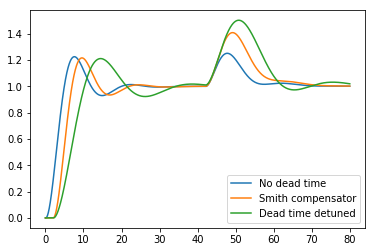
../../_images/2_Control_5_Advanced_control_methods_Dead_time_compensation_33_1.png

We see that the Smith Predictor gives us almost the same performance as the dead time free system, but that it cannot entirely compensate for the delay in the disturbance output because it doesn’t have an undelayed measurement of it. It still does better on the disturbance rejection than the detuned PI controller we had to settle for with the dead time.

[ ]: