61. Closed loop stability¶

Stability of closed loop control systems appears to be easy to determine. We can just calculate the closed loop transfer function and invert the Laplace transform.

[1]:

import sympy
sympy.init_printing()

[2]:

%matplotlib inline

[3]:

s = sympy.Symbol('s')

[4]:

K_c, t = sympy.symbols('K_c, t', positive=True)

These are the systems from Example 10.4 in Seborg et al

[5]:

G_c = K_c
G_v = 1/(2*s + 1)
G_p = G_d = 1/(5*s + 1)
G_m = 1/(s + 1)

[6]:

K_m = sympy.limit(G_m, s, 0)

[7]:

forward = G_c*G_v*G_p
backward = G_m

G_CL = K_m*forward/(1 + forward*backward)

[8]:

sympy.simplify(G_CL)

[8]:

$$\frac{K_{c} \left(s + 1\right)}{K_{c} + \left(s + 1\right) \left(2 s + 1\right) \left(5 s + 1\right)}$$

[9]:

y = G_CL/s

Now for the moment of truth. Uncomment the next line if you have a lot of time on your hands…

[10]:

#yt = sympy.inverse_laplace_transform(y, s, t)

So that didn’t really work as we expected. Can we at least calculate the roots of the denominator?

[11]:

ce = sympy.denom(G_CL.simplify())
ce.expand()

[11]:

$$K_{c} + 10 s^{3} + 17 s^{2} + 8 s + 1$$

[12]:

roots = sympy.solve(ce, s)

OK, that approach works, but is limited in the analytic case to 4th order polynomials

[13]:

sympy.plot(*[sympy.re(r) for r in roots], (K_c, 1, 20))

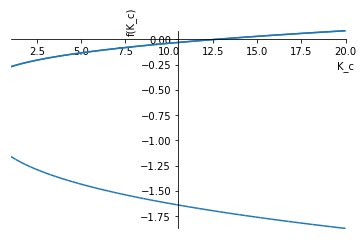
../../_images/2_Control_2_Laplace_domain_analysis_of_control_systems_Stability_analysis_17_0.png

[13]:

<sympy.plotting.plot.Plot at 0x11b5e0978>

We can see that one root gets a positive real part around $K_c=12.5$

62. Using the control library¶

We quickly run out of SymPy’s abilities when calculating closed loop transfer functions. Let’s try to do it with the control library instead:

[14]:

import control
import numpy
import scipy.signal
import matplotlib.pyplot as plt
%matplotlib inline

[15]:

s = control.tf([1, 0], [1])

[16]:

G_v = 1/(2*s + 1)
G_p = G_d = 1/(5*s + 1)
G_m = 1/(s + 1)
K_m = 1

[17]:

from tbcontrol.loops import feedback

[18]:

def closedloop(K_c):
    G_c = K_c

    G_CL = K_m*feedback(G_c*G_v*G_p, G_m)
    return G_CL

[19]:

closedloop(2)

[19]:

$$\frac{20 s^3 + 34 s^2 + 16 s + 2}{100 s^5 + 240 s^4 + 209 s^3 + 103 s^2 + 29 s + 3}$$

[20]:

from ipywidgets import interact

[21]:

smootht = numpy.linspace(0, 20)

[22]:

loop = G_v*G_p*G_m

[23]:

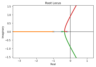
_ = control.rlocus(loop)

/Users/alchemyst/anaconda3/lib/python3.7/site-packages/matplotlib/figure.py:98: MatplotlibDeprecationWarning:
Adding an axes using the same arguments as a previous axes currently reuses the earlier instance.  In a future version, a new instance will always be created and returned.  Meanwhile, this warning can be suppressed, and the future behavior ensured, by passing a unique label to each axes instance.
  "Adding an axes using the same arguments as a previous axes "

../../_images/2_Control_2_Laplace_domain_analysis_of_control_systems_Stability_analysis_29_1.png

[24]:

def response(K_C):
    G_CL = closedloop(K_C)
    poles = G_CL.pole()
    plt.plot(*control.step_response(G_CL, smootht))
    _ = control.rlocus(loop)
    plt.scatter(poles.real, poles.imag, color='red')

[25]:

interact(response, K_C=(1., 20.))

[25]:

<function __main__.response(K_C)>

Now, the step response is calculated quickly enough that we can interact with the graphics using the slider!

62.1. Direct substitution¶

From our exploration above it is clear there is a zero of the characteristic equation at $K_C \approx 13$. Let’s solve for this numerically:

[26]:

def chareq(x):
    Kc, omega = x
    s = 1j*omega
    ce = 1 + Kc*loop
    ce_of_s = ce(s)
    return ce_of_s.real, ce_of_s.imag

[27]:

import scipy.optimize

[28]:

scipy.optimize.fsolve(chareq, [13, 1])

[28]:

array([12.6       ,  0.89442719])

How can we determine stability without calculating the roots? See the next notebook.