3. Discrete PI with ITAE parameters

This notebook reproduces Figure 17.10 in Seborg et al and also goes a little further

from tbcontrol import blocksim, fopdtitae

import numpy
import matplotlib.pyplot as plt
%matplotlib inline

def limit(u, umin, umax):
    return max(umin, min(u, umax))

class DiscretePI(blocksim.Block):
    def __init__(self, name, inputname, outputname, K, tau_I, deltat, umin=-numpy.inf, umax=numpy.inf):
        super().__init__(name, inputname, outputname)

        self.K = K
        self.tau_I = tau_I
        self.deltat = deltat
        self.umin = umin
        self.umax = umax
        self.reset()

    def reset(self):
        self.state = 0
        self.output = 0
        self.eint = 0
        self.nextsample = 0

    def change_input(self, t, e):
        if t >= self.nextsample:
            self.eint += e*self.deltat
            self.output = self.K*(e + self.eint/self.tau_I)
            self.nextsample += self.deltat

        return limit(self.output, self.umin, self.umax)

    def change_state(self, x):
        self.state = x

    def derivative(self, e):
        return 0

class DiscretePI_vel(DiscretePI):
    def reset(self):
        self.state = 0
        self.output = 0
        self.e_k_1 = 0
        self.nextsample = 0

    def change_input(self, t, e_k):
        if t >= self.nextsample:
            self.output += self.K*((e_k - self.e_k_1) + self.deltat/self.tau_I*e_k)
            self.output = limit(self.output, self.umin, self.umax)

            self.e_k_1 = e_k
            self.nextsample += self.deltat

        return self.output

The system is

\[G = G_v G_p G_m = \frac{-20 e^{-s}}{5s + 1} = \frac{K_p e^{-\theta s}}{\tau_p s + 1}\]

It is not explicitly stated in the example, but \(G_d = G\) is assumed.

Kp = -20
taup = 5
theta = 1

G = blocksim.LTI('G', 'u', 'yu',
                 Kp, [taup, 1], theta)

Gd = blocksim.LTI('G', 'd', 'yd',
                  Kp, [taup, 1], theta)

Note we can’t just do G = Gd because we need new names and a new state for the block.

sums = {'y': ('+yu', '+yd'),
        'e': ('-y', '+r')}

inputs = {'r': blocksim.zero,
          'd': blocksim.step()}

ts = numpy.linspace(0, 15, 2000)

deltats = [0.05, 0.25, 0.5, 1]

3.1. Reconstruction

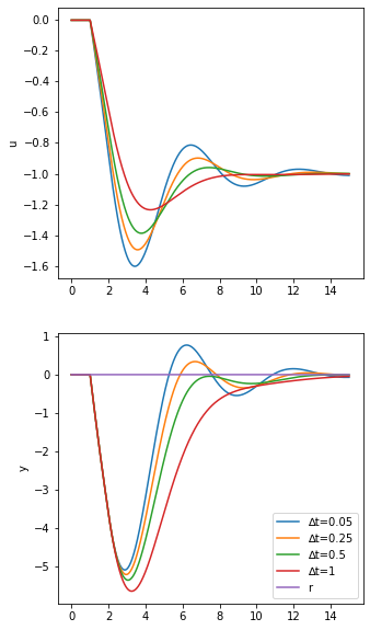
Here is the direct reconstruction of Figure 11.10. Turns out they use a continuous PI controller with the parameters for a discrete controller.

def simulate(controller, discrete=True, umin=-numpy.inf, umax=numpy.inf):
    fig, (uaxis, yaxis) = plt.subplots(2, 1, figsize=(5, 10))
    for deltat in deltats:
        Kc, tau_I = fopdtitae.parameters(Kp, taup, theta + deltat/2)
        Gc = controller('Gc', 'e', 'u',
                        Kc, tau_I,
                        *((deltat, umin, umax) if discrete else ()))
        diagram = blocksim.Diagram([G, Gd, Gc], sums, inputs)
        outputs = diagram.simulate(ts)
        uaxis.plot(ts, outputs['u'])
        yaxis.plot(ts, outputs['y'], label='∆t={}'.format(deltat))
    uaxis.set_ylabel('u')
    yaxis.set_ylabel('y')
    yaxis.plot(ts, outputs['r'], label='r')
    yaxis.legend()

simulate(blocksim.PI, discrete=False)

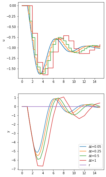
3.2. Discrete responses

simulate(DiscretePI)

simulate(DiscretePI_vel)

This looks different from the given figure, but the position form and velocity form look identical. Note that the analog PI controller gets better results than the digital approximations with the same controller parameters. “Better” in this context means that in general the error is smaller (note the worst case error in the analog case is about 5, while in the digital case it’s almost 7.

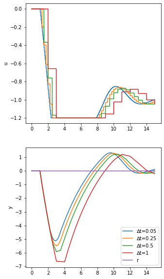
3.3. With output limits

Now, let’s include limiting behaviour

simulate(DiscretePI, umin=-1.2, umax=0)

simulate(DiscretePI_vel, umin=-1.2, umax=0)

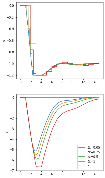
The windup on the position form PID is very clear. In the “wound up” case, the output is stuck at the limit for a long time as the controller has to unwind the integral before moving away from the limit. In the velocity form, the output comes away from the limit much faster.

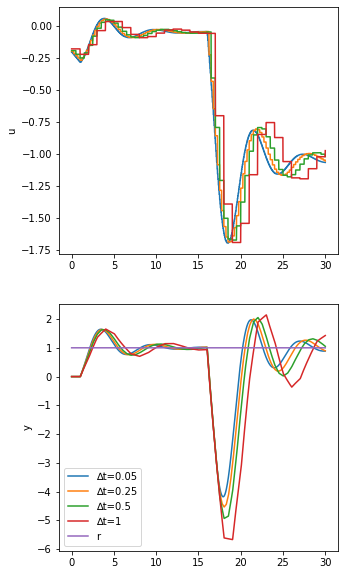
3.4. With setpoint tracking

Let’s include setpoint tracking as well.

inputs['r'] = blocksim.step(starttime=0)
inputs['d'] = blocksim.step(starttime=15)

ts = numpy.linspace(0, 30, 2000)

simulate(DiscretePI)