3. First-order system with proportional control

Consider the simple feedback loop shown below

Simple feedback loop

with $G_c=K_c$ and $G_p=\frac{1}{\tau s + 1}$

[1]:

%matplotlib inline

[2]:

import sympy
sympy.init_printing()

[3]:

G_c = K_C = sympy.Symbol('K_C', positive=True)

[4]:

s = sympy.Symbol('s')
tau = sympy.Symbol('tau', positive=True)

[5]:

G_p = 1/(tau*s + 1)
G_p

[5]:

$$\frac{1}{s \tau + 1}$$

[6]:

G_OL = G_p*G_c

[7]:

from tbcontrol.loops import feedback

The target is to get $y_{SP} = y$

[8]:

G_CL = feedback(G_OL, 1).cancel()
G_CL

[8]:

$$\frac{K_{C}}{K_{C} + s \tau + 1}$$

[9]:

t = sympy.Symbol('t', positive=True)

[10]:

general_timeresponse = sympy.inverse_laplace_transform(sympy.simplify(G_CL/s), s, t)
general_timeresponse

[10]:

$$\frac{K_{C} \left(e^{\frac{t \left(K_{C} + 1\right)}{\tau}} - 1\right) e^{- \frac{t \left(K_{C} + 1\right)}{\tau}}}{K_{C} + 1}$$

[11]:

import numpy

[12]:

import matplotlib.pyplot as plt

[13]:

y_func = sympy.lambdify((K_C, tau, t), general_timeresponse, 'numpy')

[14]:

smootht = numpy.linspace(0, 5)

[15]:

def response(K_C=10, tau=10):
    y = y_func(K_C, tau, smootht)
    e = 1 - y
    fig, [ax_y, ax_e] = plt.subplots(2, 1)
    ax_y.plot(smootht, y)
    ax_y.axhline(1)
    ax_y.set_ylabel('Setpoint and y')

    ax_e.plot(smootht, e)
    ax_e.set_ylabel('Error')

[16]:

from ipywidgets import interact

[17]:

interact(response, K_C=(0, 100), tau=(0, 20))

[17]:

<function __main__.response(K_C=10, tau=10)>

3.1. Offset as function of gain

[18]:

r = 1/s

[19]:

y = r*G_CL

[20]:

e = r - y

Use the final value statement to obtain eventual offset:

[21]:

steady_offset = sympy.limit(s*e, s, 0)
steady_offset

[21]:

$$\frac{1}{K_{C} + 1}$$

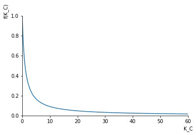
Note the steady state offset is not a function of the system dynamics (time constant).

[22]:

sympy.plot(steady_offset, (K_C, 0, 60))

../../_images/2_Control_1_Conventional_feedback_control_Effect_of_Proportional_Control_26_0.png

[22]:

<sympy.plotting.plot.Plot at 0x1141865f8>

3.2. Second order system with proportional control

[23]:

import matplotlib.pyplot as plt

[24]:

zeta = sympy.Symbol('zeta')

[25]:

G = 1/(tau**2*s**2 + 2*tau*zeta*s + 1)
G

[25]:

$$\frac{1}{s^{2} \tau^{2} + 2 s \tau \zeta + 1}$$

[26]:

G_CL = feedback(G*K_C, 1).cancel()
G_CL

[26]:

$$\frac{K_{C}}{K_{C} + s^{2} \tau^{2} + 2 s \tau \zeta + 1}$$

[27]:

def response(new_K_C, new_tau, new_zeta):
    real_CL = G_CL.subs({K_C: new_K_C, tau: new_tau, zeta: new_zeta})
    timeresponse = sympy.inverse_laplace_transform(sympy.simplify(real_CL/s), s, t)
    sympy.plot(timeresponse, 1, (t, 0, 100))
    poles = sympy.solve(sympy.denom(sympy.simplify(real_CL)), s)
    plt.plot([sympy.re(p) for p in poles], [sympy.im(p) for p in poles], 'x', markersize=10)
    plt.axhline(0, color='black')
    plt.axvline(0, color='black')
    plt.axis([-1, 1, -1, 1])

[28]:

interact(response, new_K_C=(0., 100), new_tau=(0, 10.), new_zeta=(0, 2.));

[ ]: