4. Dahlin controller

We will replicate the controller output in figure 17.11a. This notebook has a video commentary.

Note I am replicating these results using analytic methods to show that the artefacts are not numerical but rather fundamental to the calculations. If you simply want to simulate the action of a discrete controller on a continuous system, have a look at the Simple discrete controller simulation notebook.

import sympy
sympy.init_printing()
import tbcontrol
tbcontrol.expectversion('0.1.3')

5. Discretise the system

We need to find the corresponding z transform of the hold element and the system. Since \(H=1/s(1 - e^{-Ts})\), we can find \(F=G/s\), from there \(f(t)\) and then work out the \(z\) transform

s, t = sympy.symbols('s, t')
Gs = 1/(15*s**2 + 8*s + 1)
Gs

$$\frac{1}{15 s^{2} + 8 s + 1}$$

f = sympy.inverse_laplace_transform(Gs/s, s, t).simplify()
sympy.nsimplify(sympy.N(f)).simplify()

$$\theta\left(t\right) + \frac{3 e^{- \frac{t}{3}} \theta\left(t\right)}{2} - \frac{5 e^{- \frac{t}{5}} \theta\left(t\right)}{2}$$

We can see that \(f(t)\) is the sum of 1 and two exponentials. It is easy to determine the corresponding z transforms from the table

Time domain	Laplace-transform	z-transform (\(b=e^{-aT}\))
\(e^{-at}\)	\(\frac{1}{s+a}\)	\(\frac{1}{1-bz^{-1}}\)

z, q = sympy.symbols('z, q')

Now the sampling interval

T = 1 # Sampling interval

def expz(a):
    b = sympy.exp(-a*T)
    return 1/(1 - b*z**-1)

Fz = -5/2*expz(1/5)  + 3/2*expz(1/3) + 1/(1 - z**-1)

Fz

$$\frac{1.5}{1 - \frac{0.716531310573789}{z}} - \frac{2.5}{1 - \frac{0.818730753077982}{z}} + \frac{1}{1 - \frac{1}{z}}$$

Let’s see if we did that right

import tbcontrol.symbolic

def plotdiscrete(fz, N):
    values = tbcontrol.symbolic.sampledvalues(fz, z, N)
    times = [n*T for n in range(N)]
    plt.stem(times, values)

import matplotlib.pyplot as plt
%matplotlib inline

import numpy

ts = numpy.linspace(0, 10, 300)

plotdiscrete(Fz, 10)
plt.plot(ts, tbcontrol.symbolic.evaluate_at_times(f, t, ts))

[<matplotlib.lines.Line2D at 0x1205b3ef0>]

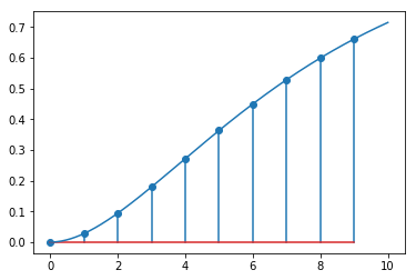
Here is the transform of the system and the hold element. See the Discrete control notebook for the derivation.

HG_z = Fz*(1 - z**-1)

6. Dahlin Controller

The desired closed loop response is first order

θ = 0 # system dead time
λ = 1 # Dahlin's lambda
h = θ # Dahlin's h

First order response in eq 17-63

N = θ/T
A = sympy.exp(-T/λ)
yclz = (1 - A)*z**(-N-1)/(1 - A*z**-1)

K = (1/HG_z*yclz/(1 - yclz)).simplify()

K

$$\frac{1.0 \left(0.632120558828558 z^{2} - 0.970470713623842 z + 0.370831136111342\right)}{0.0279700831657292 z^{2} - 0.00455601047319787 z - 0.0234140726925314}$$

#K = 0.632/(1 - z*-1) * (1 - 1.5353*z**-1 + 0.5866*z**-2)/(0.028 + 0.0234*z**-1)

We will model the control response to a unit step in reference signal

rz = 1/(1 - z**-1) # unit step in z

Now we can calculate the z-domain version of the controller output

uz = K/(1 + K*HG_z)*rz

N = 10

plotdiscrete(uz, N)

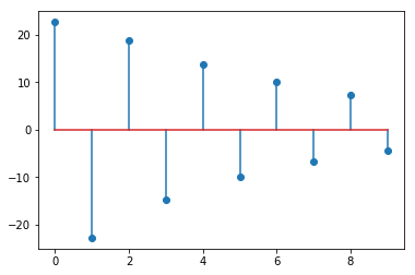
This oscillating controller output is known as “ringing”. It is an undesirable effect.

7. Continuous response

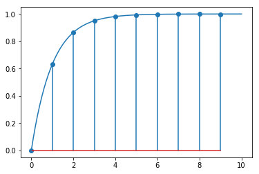
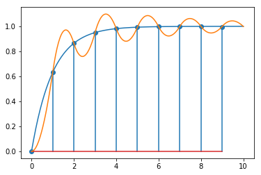
By design the controlled variable follows an exponential at the sampling points.

yz = K*HG_z/(1 + K*HG_z)*rz

plotdiscrete(yz, N)
plt.plot(ts, 1 - numpy.exp(-ts/λ))

[<matplotlib.lines.Line2D at 0x120c51390>]

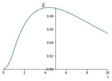
But what does it really look like between data points? First, let’s construct the response of the system to a single sampling time length pulse input

p = f - f.subs(t, t-T)

Note that there is a slight issue with finding the value of this function at zero, so we avoid that point in plotting by starting at some small value which is not zero.

smallvalue = 0.001

sympy.plot(p, (t, smallvalue, 10))

<sympy.plotting.plot.Plot at 0x1209627f0>

Let’s get the values of the controller output as a list:

u = tbcontrol.symbolic.sampledvalues(uz, z, N)

Now, we calculate the output of the system as the sum of the various pulse inputs.

yt = numpy.zeros_like(ts)
for i in range(0, N):
    yt += [float(sympy.N(u[i]*p.subs(t, ti-i + smallvalue))) for ti in ts]

Finally, we present the discrete system response, the designed response and the analytical continuous response on the same graph.

plotdiscrete(yz, 10)
plt.plot(ts, 1 - numpy.exp(-ts/λ))
plt.plot(ts, yt)

[<matplotlib.lines.Line2D at 0x12126f8d0>]