3. The \(z\)-transform

This notebook shows some techniques for dealing with discrete systems analytically using the \(z\) transform

import sympy
sympy.init_printing()

import tbcontrol
tbcontrol.expectversion('0.1.2')

s, z = sympy.symbols('s, z')
k = sympy.Symbol('k', integer=True)
Dt = sympy.Symbol('\Delta t', positive=True)

3.1. Definition

The \(z\) transform of a sampled signal (\(f^*(t)\)) is defined as follows:

\[\mathcal{Z}[f^*(t)] = \sum_{k=0}^{\infty} f(k \Delta t) z^{-k}\]

Note The notation is often abused, so you may also encounter * \(\mathcal{Z}[f(t)]\), which should be interpreted as having the sampling implied * \(\mathcal{Z}[F(s)]\), which implies that you should first calculate the inverse Laplace and then sample, so something like \(\mathcal{Z}[F(s)]=\mathcal{Z}[\mathcal{L}^{-1}[F(s)]]=\mathcal{Z}[f(t)]\) * Seborg et al use \(\mathcal{Z}[{F(s)}]\) to mean the transfer function of \(F(s)\) with a sample and zero order hold in front of it, which in these notebooks will be expressed as \(\mathcal{Z}[{H(s)F(s)}]\).

3.2. Direct calculation in SymPy

For a unit step, \(f(t)=1\) and we can obtain the \(z\) transform as an infinte series as follows:

unitstep = sympy.Sum(1 * z**-k, (k, 0, sympy.oo))
unitstep

$\displaystyle \sum_{k=0}^{\infty} z^{- k}$

Sympy can recognise this infinite series as a geometric series, and under certain conditions for convergence, it can find a finite representation:

shortform = unitstep.doit()
shortform

$\displaystyle \begin{cases} \frac{1}{1 - \frac{1}{z}} & \text{for}\: \frac{1}{\left|{z}\right|} < 1 \\\sum_{k=0}^{\infty} z^{- k} & \text{otherwise} \end{cases}$

To extract the first case solution, we use args:

uz = shortform.args[0][0]
uz

$\displaystyle \frac{1}{1 - \frac{1}{z}}$

Notice what has happened here: we have taken the infinite series and written it in a compact form. You should always keep in mind that these two forms are equivalent.

3.3. Transfer functions from difference equations

For a first order difference equation (the discrete equivalent of a first order differential equation):

\[y(k) + a_1 y(k - 1) = b_1 u(k - 1)\]

If we interpret \(z^{-n}\) as an \(n\) time step delay, can write

\[\mathcal{Z}[y(k - n)] = Y(z)z^{-n}\]

This transforms our difference equation to

\[Y(z) + a_1 z^{-1} Y(z) = b_1 z^{-1} U(z)\]

Leading to a discrete transfer function:

\[G(z) = \frac{Y(z)}{U(z)} = \frac{b_1 z^{-1}}{1 + a_1 z^{-1}}\]

Unfortunately, sympy simplifies this expression using positive powers of \(z\)

a1, b1 = sympy.symbols('a1, b1')

Gz = b1*z**-1/(1 + a1*z**-1)
Gz.cancel()

$\displaystyle \frac{b_{1}}{a_{1} + z}$

Since I have not found an easy way to get sympy to report negative powers of \(z\), I find it convenient to define

\[q = z^{-1}\]

q = sympy.symbols('q')

def qsubs(fz):
    return fz.subs({z: q**-1})

qsubs(Gz)

$\displaystyle \frac{b_{1} q}{a_{1} q + 1}$

3.4. Responses and inversion

To find the response of this system to the unit input, we can multiply the input and the transfer function. Note that this is equivalent to convolution of the polinomial coefficients.

yz = Gz*uz
qsubs(yz)

$\displaystyle \frac{b_{1} q}{\left(1 - q\right) \left(a_{1} q + 1\right)}$

Let’s evaluate that with numeric values for the coefficients:

K = 2 # The worked version in the textbook uses 2 even though the text says 20
tau = 1

Dt = 1

parameters = {a1: -sympy.exp(-Dt/tau),
              b1: K*(1 -  sympy.exp(-Dt/tau))
             }
stepresponse = yz.subs(parameters)

Remember that the \(z\) transform was defined using the values of the sampled signal at the sampling points.

\[\mathcal{Z}[f^*(t)] = \sum_{k=0}^{\infty} f(k \Delta t) z^{-k} = f(0) + f(\Delta t)z^{-1} + f(2\Delta t)z^{-2} + \cdots\]

To obtain the values of the response at the sampling points (also called inverting the \(z\) transform), we need to expand the polynomial. We can do this using Taylor series. Sympy has a Poly class which can extract all the coefficients of the polynomial easily.

N = 10

qpoly = sympy.Poly(qsubs(stepresponse).series(q, 0, N).removeO(), q)
qpoly

$\displaystyle \operatorname{Poly}{\left( 1.99975318039183 q^{9} + 1.99932907474419 q^{8} + 1.99817623606889 q^{7} + 1.99504249564667 q^{6} + 1.98652410600183 q^{5} + 1.96336872222253 q^{4} + 1.90042586326427 q^{3} + 1.72932943352677 q^{2} + 1.26424111765712 q, q, domain=\mathbb{R} \right)}$

qpoly.all_coeffs()

$\displaystyle \left[ 1.99975318039183, \ 1.99932907474419, \ 1.99817623606889, \ 1.99504249564667, \ 1.98652410600183, \ 1.96336872222253, \ 1.90042586326427, \ 1.72932943352677, \ 1.26424111765712, \ 0.0\right]$

Notice that the coefficients are returned in decreasing orders of \(q\), but we want them in increasing orders to plot them.

responses = list(reversed(qpoly.all_coeffs()))

We’ll be using this operation quite a lot so there’s a nice function in tbcontrol.symbolic that does the same thing:

import tbcontrol.symbolic

responses = tbcontrol.symbolic.sampledvalues(stepresponse, z, N)

import matplotlib.pyplot as plt
import numpy

%matplotlib inline

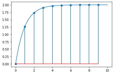
We’ll compare the values we obtained above with the step response of a continuous first order system with the same parameters:

sampledt = Dt*numpy.arange(N)

smootht = numpy.linspace(0, Dt*N)

analytic_firstorder = K*(1 - numpy.exp(-smootht/tau))

plt.stem(sampledt, numpy.array(responses, dtype=float))
plt.plot(smootht, analytic_firstorder)

[<matplotlib.lines.Line2D at 0x2a264c57388>]

3.5. Calculation using scipy

We can get the same values without going through the symbolic steps by using the scipy.signal library.

import scipy.signal

a1 = -numpy.exp(-Dt/tau)
b1 = K*(1 - numpy.exp(-Dt/tau))

Note this uses the transfer function in terms of \(z\) (not \(z^{-1}\)).

Gz.expand()

$\displaystyle \frac{b_{1}}{a_{1} + z}$

Gdiscrete = scipy.signal.dlti(b1, [1, a1], dt=1)

_, response = Gdiscrete.step(n=N)

plt.stem(sampledt, numpy.squeeze(response))
plt.plot(smootht, analytic_firstorder)

[<matplotlib.lines.Line2D at 0x2a276be5348>]

3.6. Calculation using the control libary

import control

Explicitly creating the discrete time transfer function

G = control.tf(b1, [1, a1], 1)

G

$$\frac{1.264}{z - 0.3679}\quad dt = 1$$

The discrete-time transfer function can also be sampled from the continuous transfer function

G_continuous = control.tf(K, [tau, 1])

G_continuous

$$\frac{2}{s + 1}$$

G_discrete = G_continuous.sample(1)

G_discrete

$$\frac{1.264}{z - 0.3679}\quad dt = 1$$

We continue with the explisitl transfer function (which is identical to the sampled one)

sampledt, response = control.step_response(G)

plt.stem(sampledt, numpy.squeeze(response))
plt.plot(smootht, analytic_firstorder)

[<matplotlib.lines.Line2D at 0x2a276e57188>]

I have found it useful to define

z = control.tf([1, 0], 1, 1)

z

$$\frac{z}{1}\quad dt = 1$$

This allows us to do calculations in a relatively straightforward way:

step = 1/(1 - z**-1)

step

$$\frac{z}{z - 1}\quad dt = 1$$

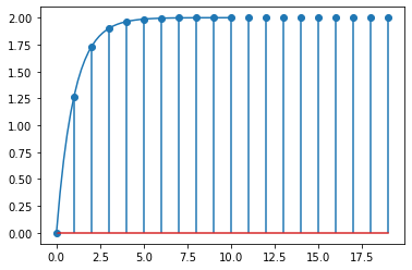
If we remember that the inversion of the signal is the same as an impulse response, we can also get the same result as follows:

sampledt, response = control.impulse_response(G*step)

plt.stem(sampledt, numpy.squeeze(response))
plt.plot(smootht, analytic_firstorder)

[<matplotlib.lines.Line2D at 0x2a277119948>]

The control library also has the capability of sampling a state space system.

Gss = control.ss(G_continuous)

Gss

A = [[-1.]]

B = [[1.]]

C = [[2.]]

D = [[0.]]

Sampling a continuous state space representation will result in a discrete-time state space representation of the system.

Gss.sample(1)

A = [[0.36787944]]

B = [[0.63212056]]

C = [[2.]]

D = [[0.]]

dt = 1

Note that MIMO functionality in the control library depends on the slycot module. In it’s current revision MIMO systems cannot be sampled. However you can sample the individual SISO systems from a transfer function matrix, and then build the discrete-time transfer function matrix, which can be converted to a state-space representation.