45. Asymptotic Bode diagrams

One of the big advantages of Bode diagrams is that they are very easy to sketch out by hand (or, equivalently, to visualise mentally).

import numpy
import matplotlib.pyplot as plt
%matplotlib inline

omega = numpy.logspace(-2, 2, 1000)
s = 1j*omega

46. Systems with real poles

Let’s study the bode diagrams of systems of the form

\[\frac{K}{(\tau s + 1)^n}\]

def annotated_bode(ax_gain, ax_phase, G, K, tau, order):
    high_freq_asymptote = K/(tau*omega)**order

    # Gain part
    ax_gain.loglog(omega, numpy.abs(G))
    ax_gain.axhline(K, color='grey')  # Rule 1
    ax_gain.loglog(omega, high_freq_asymptote, color='grey') # Rule 2
    ax_gain.axvline(1/tau, color='grey')  # Rule 2
    ax_gain.set_ylim([1e-2, 1e+1])
    ax_gain.set_ylabel('|G|')

    # Phase part
    ax_phase.axhline(0, color='grey')  # Rule 3
    ax_phase.semilogx(omega, numpy.unwrap(numpy.angle(G)))
    ax_phase.axhline(-numpy.pi/2*order, color='grey')  # Rule 4
    ax_phase.axvline(1/tau, color='grey')  # Rule 5
    ax_phase.set_ylim([-3*numpy.pi/2, 2*numpy.pi/2])
    ax_phase.set_ylabel(r'$\angle G$')

def plotresponse(order=1, tau=1, K=1):
    G = K/(tau*s + 1)**order

    fig, [ax_gain, ax_phase] = plt.subplots(2, 1)
    annotated_bode(ax_gain, ax_phase, G, K, tau, order)

from ipywidgets import interact

interact(plotresponse, order=(-2, 3), tau=(0.1, 10), K=(-1., 2));

We see that we can construct a reasonable approximation by knowing a couple of things

1. The gain (\(K\)) of the system defines the low frequency asymptote of the gain graph
2. The high frequency asymptote of the gain is \(\frac{K}{(\omega\tau)^n}\). Effectively, on a loglog scale, this means we have -n/decade slope above frequencies of around \(1/\tau\)
3. The low frequency phase asymptote is 0
4. The high frequency phase asymptote is \(-n\pi/2\)
5. The phase curve has an inflection at \(1/\tau\)

47. Systems with complex poles

Systems with complex poles show uniique frequency response behaviour. We will focus on the second order system shown below:

\[G = \frac{K}{\tau^2 s^2 + 2\tau\zeta s + 1}\]

def plotresponse(K=1, tau=1, zeta=1):
    plt.figure(figsize=(15, 5))
    order = 2
    G = K/(tau**2*s**2 + 2*tau*zeta*s + 1)

    ax_gain = plt.subplot2grid((2, 2), (0, 0))
    ax_phase = plt.subplot2grid((2, 2), (1, 0))
    ax_complex = plt.subplot2grid((2, 2), (0, 1), rowspan=2)

    annotated_bode(ax_gain, ax_phase, G, K, tau, order)

    # poles
    poles = numpy.roots([tau**2, 2*tau*zeta, 1])
    ax_complex.scatter(poles.real, poles.imag)
    ax_complex.axhline(0)
    ax_complex.axvline(0)
    ax_complex.axis([-2, 2, -2, 2])

interact(plotresponse, K=(0.1, 2), tau=(0.1, 2), zeta=(0., 1.1))

<function __main__.plotresponse(K=1, tau=1, zeta=1)>

We see that the rules from before still hold, except that we start seeing the so-called “harmonic nose” emerge when \(\zeta<\sqrt{2}/2\approx{0.7}\). The maximum of the nose occurs at the resonant frequency of

\[\omega_r = \frac{\sqrt{1 - 2\zeta^2}}{\tau}\]

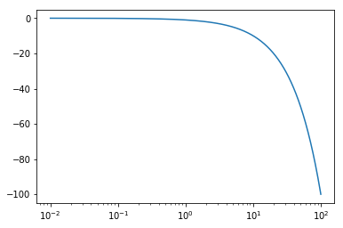
48. Dead time

The effect of dead time is to increase the phase lag indefinitely as a function of frequency. Delay has no effect on the gain of a system.

D = 1
G = numpy.exp(-D*s)

plt.semilogx(omega, numpy.unwrap(numpy.angle(G)))

[<matplotlib.lines.Line2D at 0x117a944e0>]