[1]:
import sympy
sympy.init_printing()
%matplotlib inline
1. Fourier series
We can approximate a periodic function of period P to arbitrary accuracy by adding sine and cosine terms (disguised via the Euler formula in the complex exponential):
with
Compare this last equation to the Fourier transform and the Laplace transform:
The following two functions attempt to match the notation above as closely as possible using sympy functions
[2]:
import sympy
[3]:
i2pi = sympy.I*2*sympy.pi
exp = sympy.exp
[4]:
def S(N):
    return sum(c(n)*exp(i2pi*n*t/P) for n in range(-N, N+1)).expand(complex=True).simplify()
[5]:
def c(n):
    return (sympy.integrate(
               f(t)*exp((-i2pi * n * t)/P),
               (t, t0, t0 + P))/P)
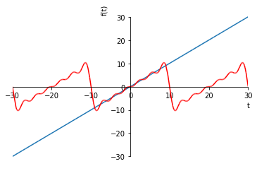
These functions work quite well for a periodic sawtooth function:
[6]:
a = sympy.Symbol('a', positive=True)
[7]:
def f(t):
    return t
[8]:
P = 20
t0 = -10
[9]:
t = sympy.Symbol('t', real=True)
[10]:
N = 6
[11]:
analytic_approx = S(N).expand()
analytic_approx
[11]:
Notice that the function we defined was just \(y=t\), but Fourier series always approximates periodic signals. We can see the bit we approximated repeating if we plot over a larger interval
[12]:
interval = (t, t0-P, t0+2*P)
p1 = sympy.plot(f(t), interval, show=False)
p2 = sympy.plot(analytic_approx, interval, show=False)
p2[0].line_color = 'red'
p1.extend(p2)
p1.show()
Unfortunately, this notationally elegant approach does not appear to work for f = sympy.Heaviside, and is also quite slow. The mpmath library supplies a numeric equivalent.
[13]:
try:
    import mpmath
except ImportError:
    from sympy import mpmath
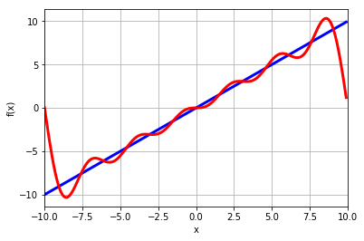
[14]:
cs = mpmath.fourier(f, [t0, t0+P], N)

def numeric_approx(t):
    return mpmath.fourierval(cs, [t0, t0+P], t)

mpmath.plot([f, numeric_approx], [t0, t0+P])
The coefficients returned by the mpmath.fourier functions are for the cosine and sine terms in this alternate representation of \(S_N\)
We can see the similarity clearly by showing the expression we obtained before multiplied out and numerically evaluated
[15]:
sympy.N(analytic_approx)
[15]:
[16]:
cs
[16]:
([mpf('0.0'),
  mpf('0.0'),
  mpf('0.0'),
  mpf('0.0'),
  mpf('0.0'),
  mpf('0.0'),
  mpf('0.0')],
 [mpf('0.0'),
  mpf('6.366197723675814'),
  mpf('-3.183098861837907'),
  mpf('2.1220659078919377'),
  mpf('-1.5915494309189535'),
  mpf('1.2732395447351628'),
  mpf('-1.0610329539459689')])
Notice that all the cosine coefficients are zero. This is true in general for odd functions.
1.1. Step function
Let’s now switch to the Heaviside step and draw the various sinusoids in the approximation more explicitly.
[17]:
import matplotlib.pyplot as plt
import numpy
%matplotlib inline
[18]:
N = 20
[19]:
@numpy.vectorize
def f(t):
    if t < 0:
        return 0
    else:
        return 1
[20]:
cs = mpmath.fourier(f, [t0, t0+P], N)
cs
[20]:
([mpf('0.5'),
  mpf('0.0'),
  mpf('0.0'),
  mpf('0.0'),
  mpf('0.0'),
  mpf('0.0'),
  mpf('0.0'),
  mpf('0.0'),
  mpf('0.0'),
  mpf('0.0'),
  mpf('0.0'),
  mpf('0.0'),
  mpf('0.0'),
  mpf('0.0'),
  mpf('0.0'),
  mpf('0.0'),
  mpf('0.0'),
  mpf('0.0'),
  mpf('0.0'),
  mpf('0.0'),
  mpf('0.0')],
 [mpf('0.0'),
  mpf('0.63675856242795037'),
  mpf('0.0002778345608862911'),
  mpf('0.21262398013873579'),
  mpf('0.00055771310594110598'),
  mpf('0.12802302327076248'),
  mpf('0.00084172518315335683'),
  mpf('0.091931640154520794'),
  mpf('0.0011320535572161288'),
  mpf('0.072015836887865267'),
  mpf('0.0014310262052054015'),
  mpf('0.059459060405769593'),
  mpf('0.0017411752581774926'),
  mpf('0.050872056499090879'),
  mpf('0.0020653060695558258'),
  mpf('0.044674904291434447'),
  mpf('0.0024065804723679999'),
  mpf('0.040032978763113902'),
  mpf('0.002768619592788056'),
  mpf('0.036465018126357898'),
  mpf('0.0031556335077388429')])
We see that all the cosine terms but the first are zero, so the first cosine coefficient represents a constant being added to the sine series.
[21]:
constant = cs[0][0]
sinecoefficients = cs[1]
I’m constructing two dimensional arrays here which will allow my formulae to work nicely when broadcasting. I’ll use the convention that the time dimension is in the columns and each sine response is in the rows.
[22]:
tt = numpy.linspace(t0, t0 + P, 1000)
t2d = tt[numpy.newaxis]  # two dimensional time array, time in the columns
[23]:
# two dimensional arrays for the sine coefficients and n - they vary in the rows
an = numpy.array(sinecoefficients)[:, numpy.newaxis]
n = numpy.arange(N+1)[:, numpy.newaxis]
This way I can build a whole array of sine responses automatically.
[24]:
sines = an*numpy.sin(2*numpy.pi*n*t2d/P)
[25]:
plt.plot(tt, f(tt))
plt.plot(tt, sines.T, color='blue', alpha=0.7)
plt.axhline(constant, color='blue', alpha=0.7)
plt.plot(tt, sum(sines) + constant)
[25]:
[<matplotlib.lines.Line2D at 0x112f5ccf8>]
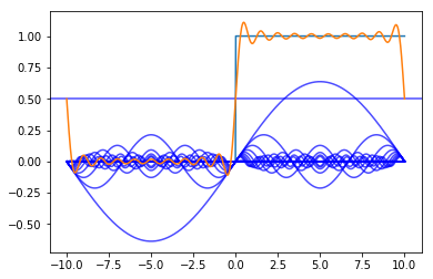
We can see that the sum of the sines approximates the step function.
1.2. Step response via Frequency response
Let’s compare the result of a “traditional” calculation of a step response of a second order system to a new way which uses the frequency response of the transfer function and the Fourier series of the step input.
First I am going to find the solution using purely analytic methods.
[26]:
s = sympy.Symbol('s')
[27]:
tau = 1
zeta = sympy.Rational(1, 2)
We redifine \(t\) here to be positive, which will allow us a simple evalutation of the inverse laplace later.
[28]:
t = sympy.Symbol('t', positive=True)
[29]:
G = 1/(tau**2*s**2 + 2*tau*zeta*s + 1)
g = sympy.inverse_laplace_transform(G/s, s, t)
Here I build a function which can evaluate the response response numerically. I use the extra argument to make the function able to work with numpy arrays
[30]:
geval = sympy.lambdify(t, sympy.N(g.simplify()), 'numpy')
[31]:
gtvalues = geval(tt)
gtvalues[tt<0] = 0
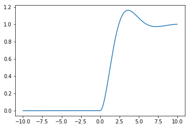
We can see the familiar second order step response:
[32]:
plt.plot(tt, gtvalues)
[32]:
[<matplotlib.lines.Line2D at 0x1130fd160>]
Now, let’s try to get the same answer by exploiting the frequency response of the transfer function. First, we need a function which can evaluate the transfer function at particular values and return a numeric result. As before I use lambdify and the extra argument to make the function able to work with numpy arrays
[33]:
Geval = sympy.lambdify(s, G, 'numpy')
Now, we need to build an array for the frequencies of the Fourier series. Remember we had terms of the form \(\sin\left(\frac{2\pi n t}{P}\right) = \sin(\omega t)\) in the Fourier series.
[34]:
omega = 2*n*numpy.pi/P
We evaluate the frequency response of the transfer function at the Fourier frequencies by using the substitution \(s=\omega i\). The complex number is j in Python.
[35]:
freqresp = Geval(omega*1j)
[36]:
K = gain = numpy.abs(freqresp)
[37]:
phi = phase = numpy.angle(freqresp)
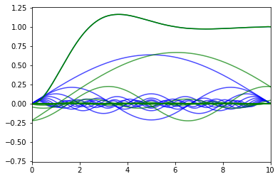
Now, we build the approximation of the respone by simply multiplying by the gain \(K\) and shifting by the phase \(\phi\):
[38]:
shiftedsines = K*an*numpy.sin(2*numpy.pi*n*t2d/P + phi)
[39]:
plt.plot(tt, gtvalues)
plt.plot(tt, sines.T, color='blue', alpha=0.7)
plt.plot(tt, shiftedsines.T, color='green', alpha=0.7)
plt.plot(tt, sum(shiftedsines) + constant, color='green')
plt.xlim(0, t0 + P)
[39]:
[ ]: