80. Simple discrete simulation: Dahlin controller

This notebook replicates Figure 17.11 in Seborg et al without using analytic methods. If you want to get some insight into the math behind the z transform, applied to the same problem see the Dahlin controller notebook.

import tbcontrol

tbcontrol.expectversion('0.2.1')

from tbcontrol import blocksim

import matplotlib.pyplot as plt
%matplotlib inline

import numpy
import control

80.1. Simple discretisation

The control module supplies an easy access point to a transfer function which represents s.

s = control.TransferFunction.s

K = 1
τ1 = 5
τ2 = 3
θ = 0

Δt = 1

assert θ % Δt == 0  # this is only correct when the delay is a multiple of the sampling time
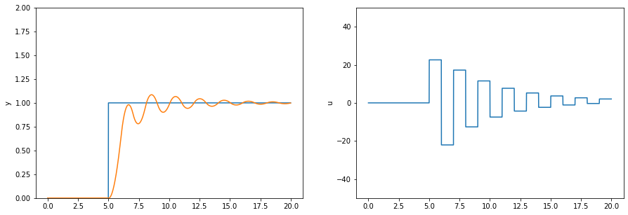
N = int(θ/Δt)

G = K/((τ1*s + 1)*(τ2*s + 1))

Discretize G assuming a zero order hold in front of it, this corresponds to using Table 17.1

z = control.TransferFunction.z

Gz = G.sample(Δt)*z**(-N)
Gz

$$\frac{0.02797 z + 0.02341}{z^2 - 1.535 z + 0.5866}\quad dt = 1$$

80.2. Do discrete transfer function math

Dahlin controller relationship

λ = Δt   # this is a tuning parameters

A = numpy.exp(-Δt/λ)
Gdc = 1/Gz * (1 - A)*z**(-N - 1) / (1 - A*z**-1 - (1 - A)*z**(-N - 1))  # eq 17.65

After these calculations Gdc is

Gdc

$$\frac{0.6321 z^4 - 0.9705 z^3 + 0.3708 z^2}{0.02797 z^4 - 0.004556 z^3 - 0.02341 z^2}\quad dt = 1$$

Notice that there are “extra” orders of z above and below the line in that expression - we could simplify it. This is what .minreal does.

Gdc = Gdc.minreal()

Gdc

$$\frac{22.6 z^2 - 34.7 z + 13.26}{z^2 - 0.1629 z - 0.8371}\quad dt = 1$$

Much better.

80.3. Convert from positive to negative powers of z

We still have a problem, though, since the control library uses positive powers of \(z\) rather than negative powers of \(z\). tbcontrol.conversion contains some methods to help convert such polynomials. Also notice that the .num and .den properties of the control library’s tf objects are designed for MIMO systems, so they are nested lists corresponding with the index of the output and the input we want. Since we’re just looking at one input and one output, we need the first element of the first element ([0][0]).

import tbcontrol.conversion

Gdc_neg_num, Gdc_neg_den = tbcontrol.conversion.discrete_coeffs_pos_to_neg(Gdc.num[0][0], Gdc.den[0][0])

Gdc_neg_num

[22.59988127611586, -34.69674036625465, 13.258134912008916]

Gdc_neg_den

[1.0, -0.1628886995509321, -0.8371113004490679]

80.4. Simple blocksim simulation

blocksim_G = blocksim.LTI('G', 'u', 'yu', G.num[0][0], G.den[0][0])

blocksim_Gdc = blocksim.DiscreteTF('Gc', 'e', 'u', 1, Gdc_neg_num, Gdc_neg_den)

diagram = blocksim.simple_control_diagram(blocksim_Gdc, blocksim_G, ysp=blocksim.step(starttime=5))

ts = numpy.arange(0, 20, 0.01)

result = diagram.simulate(ts)

def plot_outputs(result):
    fig, (ax_y, ax_u) = plt.subplots(1, 2, figsize=(15, 5))

    ax_y.plot(ts, result['ysp'])
    ax_y.plot(ts, result['y'])
    ax_y.set_ylim(0, 2)
    ax_y.set_ylabel('y')

    ax_u.plot(ts, result['u'])
    ax_u.set_ylim(-50, 50)
    ax_u.set_ylabel('u')

plot_outputs(result)