1. Multivariable control

You may want to review the Transfer function matrix notebook before you look at this one.

1.1. Closed loop transfer functions for multivariable systems

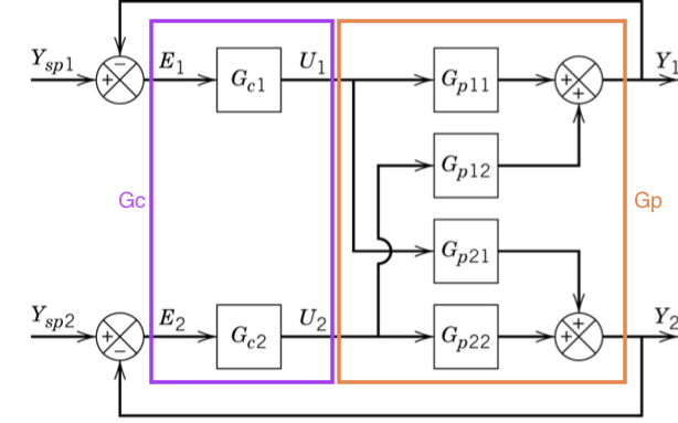
Let’s consider a 2 \(\times\) 2 system with feedback control as shown below:

import sympy
sympy.init_printing()

G_p11, G_p12, G_p21, G_p22, G_c1, G_c2 = sympy.symbols('G_p11, G_p12, G_p21, G_p22, G_c1, G_c2')

The matrix representation of the system is straigtforwardly handled by sympy.Matrix:

G_p = sympy.Matrix([[G_p11, G_p12],
                    [G_p21, G_p22]])

The controller is a bit harder. Convince yourself you understand how the off-diagonal elements of \(G_c\) are zero in the diagram above.

G_c = sympy.Matrix([[G_c1, 0],
                    [0, G_c2]])

Now, we can redraw the block diagram using vectors for the signals and matrices for the blocks.

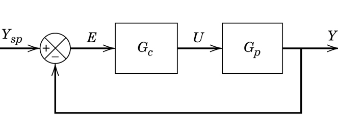
Let’s derive the closed loop transfer function. There are three equations represented in the above diagram:

\begin{align} E &= Y_{sp} - Y\\ U &= G_c E = G_c(Y_{sp} - Y)\\ Y &= G_p U = G_p G_c(Y_{sp} - Y)\\ \end{align}

Now, we can solve for \(Y\):

:nbsphinx-math:`begin{align} Y &= G_p G_c(Y_{sp} - Y)\ Y &= G_p G_c Y_{sp} - G_p G_c Y \ Y + G_p G_c Y&= G_p G_c Y_{sp} \ (I + G_p G_c) Y &= G_p G_c Y_{sp} \

Y &= (I + G_p G_c)^{-1} G_p G_c Y_{sp} \ Y &= Gamma Y_{sp}

end{align}`

We can calculate the value of this function easily.

I = sympy.Matrix([[1, 0],
                  [0, 1]])

Gamma = sympy.simplify((I + G_p*G_c).inv()*G_p*G_c)

Gamma[0, 0]

$$\frac{G_{c1} \left(G_{c2} G_{p12} G_{p21} - G_{p11} \left(G_{c2} G_{p22} + 1\right)\right)}{G_{c1} G_{c2} G_{p12} G_{p21} - \left(G_{c1} G_{p11} + 1\right) \left(G_{c2} G_{p22} + 1\right)}$$

Gamma[0, 1]

$$- \frac{G_{c2} G_{p12}}{G_{c1} G_{c2} G_{p12} G_{p21} - \left(G_{c1} G_{p11} + 1\right) \left(G_{c2} G_{p22} + 1\right)}$$

We notice that there is a common divisor in all the elements of \(\Gamma\). This is due to the calculation of the inverse of \((I + G_p G_c)\), which involves calculation of the determinant \(|I + G_p G_c|\).

Delta = (I + G_p*G_c).det()
Delta

$$G_{c1} G_{c2} G_{p11} G_{p22} - G_{c1} G_{c2} G_{p12} G_{p21} + G_{c1} G_{p11} + G_{c2} G_{p22} + 1$$

(Delta*Gamma).simplify()

$$\left[\begin{matrix}G_{c1} \left(G_{c2} G_{p11} G_{p22} - G_{c2} G_{p12} G_{p21} + G_{p11}\right) & G_{c2} G_{p12}\\G_{c1} G_{p21} & G_{c2} \left(G_{c1} G_{p11} G_{p22} - G_{c1} G_{p12} G_{p21} + G_{p22}\right)\end{matrix}\right]$$

1.2. Characteristic equation

This leads us to conclude that we can calculate the characteristic equation of the closed loop transfer function as \(|I + G_p G_c|\).

Notice that if we wanted the coupling the other way around, we could have worked with the same controller matrix permuted:

G_c*sympy.Matrix([[0, 1], [1, 0]])

$$\left[\begin{matrix}0 & G_{c1}\\G_{c2} & 0\end{matrix}\right]$$