3. Multivariable pairing (RGA)

For a 2$:nbsphinx-math:`times`$2 system, we have 2 choices of pairing variables for distributed control:

Diagonal	Off-diagonal
\[\begin{split}G_{cd} = \left[\begin{array}{cc} G_{c1} & 0 \\ 0 & G_{c2} \end{array}\right]\end{split}\]	\[\begin{split}G_{co} = \left[\begin{array}{cc} 0 & G_{c2} \\ G_{c1} & 0 \end{array}\right]\end{split}\]

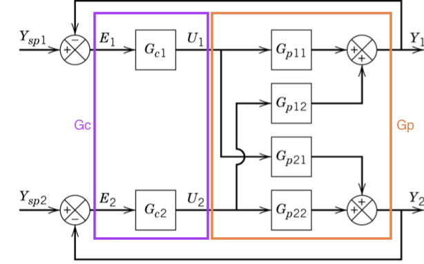
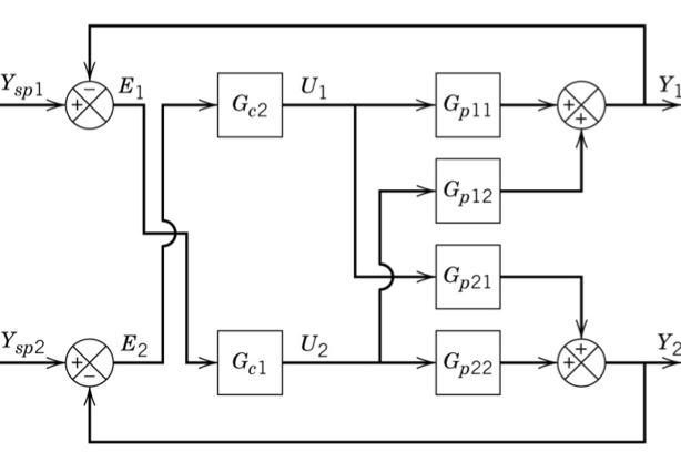
Bristol developed the Relative Gain Array to determine good pairings based on only the plant transfer function matrix \(G_p\). The elements of the RGA are defined as

\[\lambda_{ij} \triangleq \frac{(\partial y_i/\partial u_j)_u}{(\partial y_i/\partial u_j)_y}= \frac{\text{open loop gain}}{\text{closed loop gain}}\]

We could build \(\Lambda\) by direct evaluation of the above derivatives near some point given a time-domain model, but if we already have a transfer function model, we can evaluate the steady-state gain matrix \(K\) by using the final value theorem.

import sympy
sympy.init_printing()

s = sympy.Symbol('s')

def fopdt(k, theta, tau):
    return k*sympy.exp(-theta*s)/(tau*s + 1)

Using the system from example 16.5

G_p = sympy.Matrix([[fopdt(-2, 1, 10), fopdt(1.5, 1, 1)],
                    [fopdt(1.5, 1, 1), fopdt(2, 1, 10)]])
G_p

$$\left[\begin{matrix}- \frac{2 e^{- s}}{10 s + 1} & \frac{1.5 e^{- s}}{s + 1}\\\frac{1.5 e^{- s}}{s + 1} & \frac{2 e^{- s}}{10 s + 1}\end{matrix}\right]$$

Unfortunately sympy cannot calculate limits on matrix expressions

#K = sympy.limit(G_p, s, 0)

But we can apply a function to the elements:

def gain(G):
    return sympy.limit(G, s, 0)

K = G_p.applyfunc(gain)

K

$$\left[\begin{matrix}-2 & 1.5\\1.5 & 2\end{matrix}\right]$$

We can then calculate \(\Lambda = K \otimes H\) where \(H = (K^{-1})^{T}\):

Lambda = K.multiply_elementwise(K.inv().transpose())
Lambda

$$\left[\begin{matrix}0.64 & 0.36\\0.36 & 0.64\end{matrix}\right]$$

We can do the same calculation (faster) using numpy:

import numpy

def fopdt(k, theta, tau):
    return k*numpy.exp(-theta*s)/(tau*s + 1)

s = 0

K = numpy.matrix([[fopdt(-2, 1, 10), fopdt(1.5, 1, 1)],
                  [fopdt(1.5, 1, 1), fopdt(2, 1, 10)]])

The .A attribute in matrices is the matrix as a numpy.array, which multiplies elementwise by default.

K.A*K.I.T.A

array([[0.64, 0.36],
       [0.36, 0.64]])

The numpy developers recommended that you should use numpy.array instead of numpy.matrix as much as possible. I find this makes the notation harder to read:

K = numpy.array([[fopdt(-2, 1, 10), fopdt(1.5, 1, 1)],
                 [fopdt(1.5, 1, 1), fopdt(2, 1, 10)]])

K*numpy.linalg.inv(K).T

array([[0.64, 0.36],
       [0.36, 0.64]])

3.1. Simulation results

Let’s simulate this system to get an idea of how the control works out

import tbcontrol
tbcontrol.expectversion('0.1.4')
from tbcontrol import blocksim

import numpy

N = 2

G = {}

gains = [[-2, 1.5],
         [1.5, 2]]
taus = [[10, 1],
        [1, 10]]
delays = [[1, 1],
          [1, 1]]

for inp in range(N):
    for outp in range(N):
        G[(outp, inp)] = blocksim.LTI(f"G_{outp}_{inp}", f"u_{inp}", f"yp_{inp}_{outp}",
                                      gains[outp][inp], [1, taus[outp][inp]], delays[outp][inp])

inputs = {'ysp_0': blocksim.step(),
          'ysp_1': blocksim.step(starttime=50)}

sums = {f'y_{outp}': [f"+yp_{inp}_{outp}" for inp in range(N)] for outp in range(N)}
for i in range(N):
    sums[f'e_{i}'] = [f'+ysp_{i}', f'-y_{i}']

sums

{'y_0': ['+yp_0_0', '+yp_1_0'],
 'y_1': ['+yp_0_1', '+yp_1_1'],
 'e_0': ['+ysp_0', '-y_0'],
 'e_1': ['+ysp_1', '-y_1']}

import matplotlib.pyplot as plt
%matplotlib inline

def simulate(auto1=True, K1=-1, tauI1=10, auto2=True, K2=0.5, tauI2=10):
    controllers = {'Gc_0': blocksim.PI('Gc_0', 'e_0', 'u_0', K1, tauI1),
                   'Gc_1': blocksim.PI('Gc_1', 'e_1', 'u_1', K2, tauI2)}

    controllers['Gc_0'].automatic = auto1
    controllers['Gc_1'].automatic = auto2

    ts = numpy.arange(0, 100, 0.125)

    diagram = blocksim.Diagram(list(G.values()) + list(controllers.values()), sums, inputs)

    result = diagram.simulate(ts)

#     plt.figure()
#     plt.plot(ts, result['u_0'])
#     plt.plot(ts, result['u_1'])

    plt.figure()
    plt.plot(ts, result['y_0'])
    plt.plot(ts, result['ysp_0'])
    plt.plot(ts, result['y_1'])
    plt.plot(ts, result['ysp_1'])

from ipywidgets import interact

interact(simulate,
         auto1=[True, False], K1=(-2., 0), tauI1=(1., 50),
         auto2=[True, False], K2=(0., 2), tauI2=(1., 50))

<function __main__.simulate(auto1=True, K1=-1, tauI1=10, auto2=True, K2=0.5, tauI2=10)>