5. Visualising complex functions

5.1. One-dimensional functions

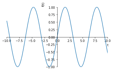
Consider a “normal” plot of \(\sin(t)\):

import sympy
sympy.init_printing()

%matplotlib inline

t = sympy.Symbol('t')

sympy.plot(sympy.sin(t))

<sympy.plotting.plot.Plot at 0x10f372470>

This allows us to see exactly what the of \(\sin(t)\) is for every value of \(t\). To do this, we need two dimensions: one for the value of \(t\) and one for \(\sin(t)\).

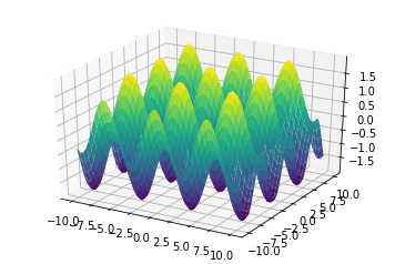
If we want to plot a function of two variables we start needing three dimensions. The following plot shows a “fake” 3d plot. It’s fake because in fact there are only two dimensions available on your computer screen. So we’re already in a bit of trouble when trying to visualise the relationships represented by higher dimensional functions.

x, y = sympy.symbols('x, y')

f2 = sympy.sin(x) + sympy.cos(y)

sympy.plotting.plot3d(f2)

<sympy.plotting.plot.Plot at 0x1113c2320>

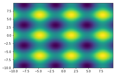
We can make up for some of this lack by using colors to represent another axis.

import numpy
import matplotlib.pyplot as plt

f2numeric = sympy.lambdify((x, y), f2, 'numpy')

xx, yy = numpy.mgrid[-10:10:0.1, -10:10:0.1]

zz = f2numeric(xx, yy)

plt.pcolor(xx, yy, zz)

<matplotlib.collections.PolyCollection at 0x111922550>

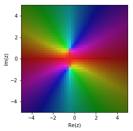
For transfer functions, we have an even bigger challenge, because we have two input variables (the real and imaginary part of \(s\)) and two output variables (the real and imaginary part of \(G(s)\)). One solution to the problem is to use colors for \(\angle G(s)\) and brightness for \(|G(s)|\). This is known as domain colouring and is supplied by mpmath.cplot.

try:
    import mpmath
except:
    from sympy import mpmath

s = sympy.Symbol('s')

G = 1/(s**2 + s + 1)
Gnumeric = sympy.lambdify(s, G)
mpmath.cplot(Gnumeric)

We can get a smoother result by plotting with more points

mpmath.cplot(Gnumeric, points=10000)

The roots of the denominator appear as two bright regions.

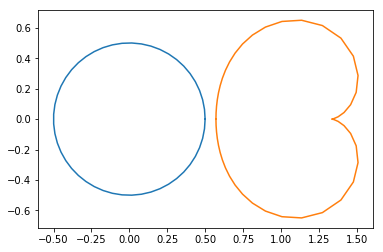
Another solution is to plot the image of \(G(s)\) as \(s\) goes through a particular path. We will speak more of this when we cover the frequency domain, but have a look at this example. We generate values of \(s\) in a circle of diameter 1 (radius 0.5) around the origin, then plot \(G(s)\) for all these \(s\) values. This is known as the image of \(G(s)\) for these values of \(s\).

theta = numpy.linspace(0, 2*numpy.pi)  # angles around the circle
s = 0.5*(numpy.cos(theta) + numpy.sin(theta)*1j) # The circle with radius 0.5
Gs = Gnumeric(s)

plt.plot(s.real, s.imag)
plt.plot(Gs.real, Gs.imag)
plt.axis('equal');