We covered the idea of simulating an arbitrary transfer function system in a previous notebook. What happens if we have to simulate a controller (specified as a transfer function) and a system specified by differential equations together?

3. Nonlinear tank system

Let’s take the classic tank system, with a square root flow relationship on the outflow and a nonlinear valve relationship.

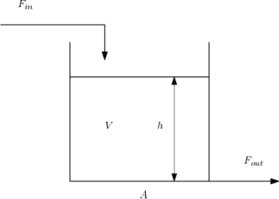
:nbsphinx-math:`begin{align}

frac{dV}{dt} &= (F_{in} - F_{out}) \ h &= frac{V}{A} \ f(x) &= alpha^{x - 1} \ F_{out} &= K f(x) sqrt{h} \

end{align}`

import numpy
import matplotlib.pyplot as plt
%matplotlib inline

Parameters

A = 2
alpha = 20
K = 2

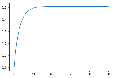
Initial conditions (notice I’m not starting at steady state)

Fin = 1
h = 1
V = A*h
x0 = x = 0.7

Valve characterisitic

def f(x):
    return alpha**(x - 1)

Integration time

ts = numpy.linspace(0, 100, 1000)
dt = ts[1]

Notice that I have reordered the equations here so that they can be evaluated in order to find the volume derivative.

hs = []
for t in ts:
    h = V/A
    Fout = K*f(x)*numpy.sqrt(h)
    dVdt = Fin - Fout
    V += dVdt*dt

    hs.append(h)

plt.plot(ts, hs)

[<matplotlib.lines.Line2D at 0x10e93ca20>]

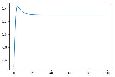
4. PI Control

Now we can include a controller controlling the level by manipulating the valve fraction

import scipy.signal

Let’s do a PI controller:

\[G_c = K_c(1 + \frac{1}{\tau_I s}) = \frac{K_C \tau_I s + K_Cs^0}{\tau_I s + 0s^0}\]

Kc = -1
tau_i = 5

In versions of scipy < 1.0, Gc would automatically have a .A attribute. After 1.0, we need to convert to state space explicitly with .to_ss().

Gc = scipy.signal.lti([Kc*tau_i, Kc], [tau_i, 0]).to_ss()

hsp = 1.3

V = 1
hs = []
xc = numpy.zeros([Gc.A.shape[0], 1])
for t in ts:
    h = V/A
    e = hsp - h  # we cheat a little here - the level we use to calculate the error is from the previous time step

    # e is in the input to the controller, yc is the output
    dxcdt = Gc.A.dot(xc) + Gc.B.dot(e)
    yc = Gc.C.dot(xc) + Gc.D.dot(e)

    x = x0 + yc[0,0]  # x0 is the controller bias

    Fout = K*f(x)*numpy.sqrt(h)
    dVdt = Fin - Fout

    V += dVdt*dt
    xc += dxcdt*dt

    hs.append(h)

plt.plot(ts, hs)

[<matplotlib.lines.Line2D at 0x1c1a0f31d0>]