1. Standard process inputs

import sympy
import matplotlib.pyplot as plt
sympy.init_printing()
%matplotlib inline

1.1. Step

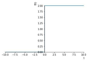
A step input of magnitude \(M\) can be written as

\[\begin{split}u_S(t)=\begin{cases} 0& t<0,\\ M& t\geq 0 \end{cases}\end{split}\]

Sympy supplies a unit step function called Heaviside, which is typeset as \(\theta(t)\)

t = sympy.symbols('t')

S = sympy.Heaviside

M = 2

sympy.plot(M*S(t))

<sympy.plotting.plot.Plot at 0x1178f46a0>

1.2. Laplace transform

Sympy can calculate laplace transforms of the step easily:

M, s = sympy.symbols('M, s')

def L(f):
    return sympy.laplace_transform(f, t, s, noconds=True)
def invL(F):
    return sympy.inverse_laplace_transform(F, s, t)

L(M*S(t))

$$\frac{M}{s}$$

1.3. Scaling and translation

We can scale and translate the step function in the normal way. Notice that how the time translation is handled.

from ipywidgets import interact

def translated_step(scale, y_translation, t_translation):
    f = scale*S(t - t_translation) + y_translation
    print("f =", f, "  \u2112(f) =", L(f))
    sympy.plot(f, (t, -10, 10), ylim=(-2, 4))

interact(translated_step,
         scale=(0.5, 3.),
         y_translation=(-1., 1.),
         t_translation=(0., 5.));

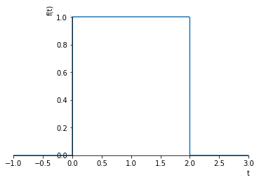
1.4. Rectangular pulse

It is now easy to see how we can construct a rectangular pulse, of height \(h\) and width \(t_w\),

\[\begin{split}u_{RP}(t)=\begin{cases} 0& t<0,\\ h& 0 \leq t < t_w\\ 0& t \geq t_w \end{cases}\end{split}\]

by using shifted versions of the step, so that

h, t_w = sympy.symbols('h, t_w')
u_RP = h*(S(t - 0) - S(t - t_w))

sympy.plot(u_RP.subs({h: 1, t_w: 2}), (t, -1, 3));

L(u_RP)

$$\frac{h}{s} - \frac{h}{s} e^{- s t_{w}}$$

1.4.1. Arbitrary piecewise constant functions

We can constuct any piecewise constant function by adding together step functions shifted in time. As an example, we can take the function represented below:

x = [-1, 0, 0, 1, 1, 2, 2, 3]
y = [0, 0, 1, 1, 2, 2, 0, 0]

plt.plot(x, y)
plt.text(0, 0.5, r'$\Delta_1=1$')
plt.text(1, 1.5, r'$\Delta_2=1$')
plt.text(2, 1, r'$\Delta_3=-2$')

plt.text(0, 0.1, r'$D_1=0$')
plt.text(1, 0.1, r'$D_2=1$')
plt.text(2, 0.1, r'$D_3=2$')

Text(2,0.1,'$D_3=2$')

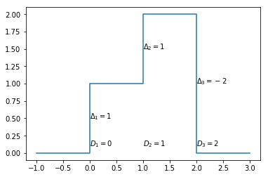
In general piecewise constant functions like the one above can be written as

\[f_c(t) = \sum_{i=1}^{N_d} \Delta_i S(t - D_i)\]

where \(S\) is the unit step. We calculate \(\Delta_i\) as the difference between the values at the discontinuities, positive if the function is rising and negative if it is falling. \(D_i\) is the time at which the value changes and \(N_d\) is the number of discontinuities.

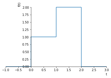
We can apply this directly for the example function.

f = 1*S(t) + 1*S(t-1) - 2*S(t-2)
f

$$\theta\left(t\right) - 2 \theta\left(t - 2\right) + \theta\left(t - 1\right)$$

Or a little more generally using some code:

Delta = [1, 1, -2]
D = [0, 1, 2]
Nd = len(Delta)

f = sum(Delta[i]*S(t - D[i]) for i in range(Nd))

f

$$\theta\left(t\right) - 2 \theta\left(t - 2\right) + \theta\left(t - 1\right)$$

Let’s verify it works properly:

sympy.plot(f, (t, -1, 3));

sympy.expand(L(f))

$$\frac{1}{s} + \frac{e^{- s}}{s} - \frac{2}{s} e^{- 2 s}$$

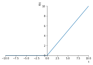
1.5. Ramp

A ramp with slope \(a\) can be written as

\[\begin{split}u_R(t)=\begin{cases} 0& t<0,\\ a& t\geq 0 \end{cases}\end{split}\]

We can construct a unit (\(a=1\)) ramp by simply multiplying the unit step by \(t\)

def R(t):
    return t*S(t)

sympy.plot(R(t))

<sympy.plotting.plot.Plot at 0x11a539198>

L(R(t))

$$\frac{1}{s^{2}}$$

1.6. Continuous piecewise linear functions

We can build any continuous piecewise linear function by using shifted and scaled ramps.

\[f(t) = \sum_{i=1}^{N_s} \Delta m_i R(t - D_{s,i})\]

This time \(\Delta m_i\) represents changes in slopes (\(m=\frac{\Delta y}{\Delta x}\)). \(D_{s,i}\) are the times at which the slopes change and \(N_s\) is the number of slope changes.

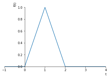
For instance, we can construct a triangular pulse by adding three ramps together.

r1 = t*S(t - 0)
r2 = -2*(t - t_w/2)*S(t - t_w/2)
r3 = (t - t_w)*S(t - t_w)
u_TP = 2/t_w*(r1 + r2 + r3)

u_TP

$$\frac{2}{t_{w}} \left(t \theta\left(t\right) + \left(- 2 t + t_{w}\right) \theta\left(t - \frac{t_{w}}{2}\right) + \left(t - t_{w}\right) \theta\left(t - t_{w}\right)\right)$$

sympy.plot(u_TP.subs({t_w: 2}), (t, -1, 4))

<sympy.plotting.plot.Plot at 0x11a6de550>

L(u_TP.subs({t_w: 2})).expand()

$$\frac{1}{s^{2}} - \frac{2}{s^{2}} e^{- s} + \frac{1}{s^{2}} e^{- 2 s}$$

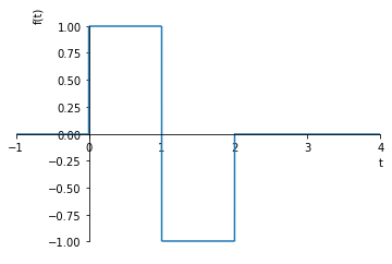
Notice that there are three ramps here (one may have expected only two). It becomes more clear when we think about the derivative of this function:

sympy.plot(u_TP.diff(t).subs({t_w: 2}), (t, -1, 4), ylim=(-1.1, 1.1))

<sympy.plotting.plot.Plot at 0x11c5a5710>

We now see that the derivative of a piecewise linear continuous function is a piecewise constant function. We can apply our rule for piecewise constant functions and integrate the steps to ramps:

derivative = 1*S(t-0) - 2*S(t-1) + 1*S(t-2)

final = 1*R(t-0) - 2*R(t-1) + 1*R(t-2)

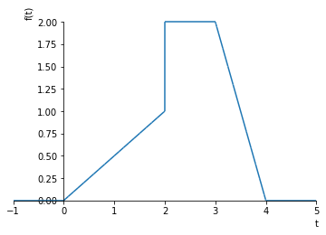
1.7. Arbitrary piecewise linear functions

We can construct any piecewise linear function by adding together ramp functions and steps shifted in time. The general rule now becomes

\[f(t) = \underbrace{\sum_{i=1}^{N_s} \Delta m_i R(t - D_{s,i})}_\text{slope changes} + \underbrace{\sum_{i=1}^{N_d} \Delta_i S(t - D_i)}_\text{discontinuities}\]

x = [-1, 0, 2, 2, 3, 4, 5]
y = [0, 0, 1, 2, 2, 0, 0]

plt.plot(x, y)

[<matplotlib.lines.Line2D at 0x11ac04d30>]

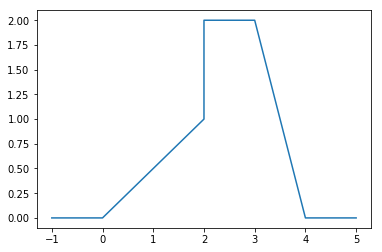
We see that there are 4 slope changes (at t=0, t=2, t=3 and t=4) and 1 discontinuity. Applying our formula yields:

g = 0.5*R(t) - 0.5*R(t-2) - 2*R(t-3) + 2*R(t - 4) + S(t - 2)

sympy.plot(g, (t, -1, 5));

sympy.expand(L(g))

$$\frac{1.0}{s} e^{- 2 s} + \frac{0.5}{s^{2}} - \frac{0.5}{s^{2}} e^{- 2 s} - \frac{2.0}{s^{2}} e^{- 3 s} + \frac{2.0}{s^{2}} e^{- 4 s}$$