2. Minimal integral measures
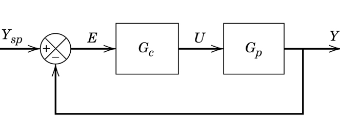
One approach to finding controller parameters is to minimise some error measure with respect to the parameters. We will simulate a first order plus dead time system under PI control. The block diagram here is for simple feedback:
[1]:
import numpy
import scipy.signal
import scipy.optimize
import matplotlib.pyplot as plt
from tbcontrol import blocksim
%matplotlib inline
[2]:
# This is the 1,1 element of a Wood and Berry column (see eq 16-12)
K = 12.8
tau = 16.7
theta = 1
[3]:
ts = numpy.linspace(0, 2*tau, 500)
[4]:
ysp = 1
[5]:
Kc = 1
tau_i = 1
[6]:
def response(Kc, tau_i):
    Gp = blocksim.LTI('G', 'u', 'y', [K], [tau, 1], theta)
    Gc = blocksim.PI('Gc', 'e', 'u', Kc, tau_i)

    blocks = [Gp, Gc]
    inputs = {'ysp': lambda t: ysp}
    sums = {'e': ('+ysp', '-y')}

    diagram = blocksim.Diagram(blocks, sums, inputs)

    return numpy.array(diagram.simulate(ts)['y'])
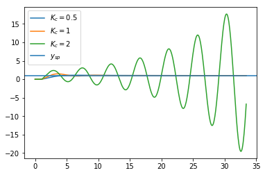
What does the setpoint response look like?
[7]:
for Kc in [0.5, 1, 2]:
    plt.plot(ts, response(Kc, 10), label='$K_c={}$'.format(Kc))
plt.axhline(ysp, label='$y_{sp}$')
plt.legend()
[7]:
<matplotlib.legend.Legend at 0x15e823d10>
These are the error measures in the book (eq 11-35 to 11-37). Note that the syntax f(*parameters) with parameters=(1, 2) is equivalent to f(1, 2).
[8]:
def iae(parameters):
    return scipy.integrate.trapezoid(numpy.abs(response(*parameters) - ysp), ts)
[9]:
def ise(parameters):
    return scipy.integrate.trapezoid((response(*parameters) - ysp)**2, ts)
[10]:
def itae(parameters):
    return scipy.integrate.trapezoid(numpy.abs(response(*parameters) - ysp)*ts, ts)
[11]:
errfuns = {'IAE': iae, 'ISE': ise, 'ITAE': itae}
Now we can find the optimal parameters for the various error measures.
[12]:
optimal_parameters = {}
for name, error in errfuns.items():
    optimal_parameters[name] = scipy.optimize.minimize(error, [1, 10]).x
    print(name, *optimal_parameters[name])
    plt.plot(ts, response(*optimal_parameters[name]), label=name)
plt.axhline(1, label='setpoint')
plt.legend(loc='best')
IAE 0.6639473997651734 16.699299499220437
ISE 0.8519788150983427 25.497869560035465
ITAE 0.5856443504019271 16.700012698516577
[12]:
<matplotlib.legend.Legend at 0x15e8ccf90>

We could also have used table 11.3, which is automated by a function in tbcontrol (see the ITAE parameters for FOPDT system notebook for more information on this function)
[13]:
from tbcontrol.fopdtitae import parameters
[14]:
Kc, tau_i = parameters(K, tau, theta, "Set point", "PI")

print(Kc, tau_i)
0.6035259299979403 16.370626907724816
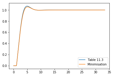
These values correspond approximately with those found through direct minimisation.
[15]:
plt.plot(ts, response(Kc, tau_i), label='Table 11.3')
plt.plot(ts, response(*optimal_parameters['ITAE']), label='Minimisation')
plt.legend()
[15]:
<matplotlib.legend.Legend at 0x15ec403d0>
[16]:
itae([Kc, tau_i])
[16]:
4.025429557262326
[17]:
itae(optimal_parameters['ITAE'])
[17]:
3.6448746068411344
Note that the error we obtained via direct minimisation was lower than the one obtained via the table, as they have fitted a curve through the results.