5. Decoupling

Given a general multivariable system with transfer function matrix \(G_p\), a decoupler attempts to combine with the system to form a diagonal whole.

import sympy
sympy.init_printing()

G_p11, G_p12, G_p21, G_p22 = sympy.symbols('G_p11, G_p12, G_p21, G_p22')
G_p = sympy.Matrix([[G_p11, G_p12],[G_p21, G_p22]])
G_p

$$\left[\begin{matrix}G_{p11} & G_{p12}\\G_{p21} & G_{p22}\end{matrix}\right]$$

5.1. 1. Inverse-based

Wouldn’t it be nice if the system didn’t have interaction? In other words, we could choose \(T\) such that we have this system with the same diagonal elements as the original system but zeros in the off diagonals.

G_s = sympy.Matrix([[G_p11, 0],[0, G_p22]])
G_s

$$\left[\begin{matrix}G_{p11} & 0\\0 & G_{p22}\end{matrix}\right]$$

Recalling that the combination of \(T\) and \(G_p\) in series is \(G_p T\), we can solve for the decoupler directly

\[G_P T = G_s \therefore T = G_P^{-1} G_s\]

T = G_p.inv()*G_s
T

$$\left[\begin{matrix}\frac{G_{p11} G_{p22}}{G_{p11} G_{p22} - G_{p12} G_{p21}} & - \frac{G_{p12} G_{p22}}{G_{p11} G_{p22} - G_{p12} G_{p21}}\\- \frac{G_{p11} G_{p21}}{G_{p11} G_{p22} - G_{p12} G_{p21}} & \frac{G_{p11} G_{p22}}{G_{p11} G_{p22} - G_{p12} G_{p21}}\end{matrix}\right]$$

Let’s see if that worked:

G_pT = G_p*T
sympy.simplify(G_pT)

$$\left[\begin{matrix}G_{p11} & 0\\0 & G_{p22}\end{matrix}\right]$$

Pros:

• Controller design can be based on open loop model

• Apparent dynamics (what the controller sees) are simple

Cons:

• T is often not physically realisable

• T is complicated

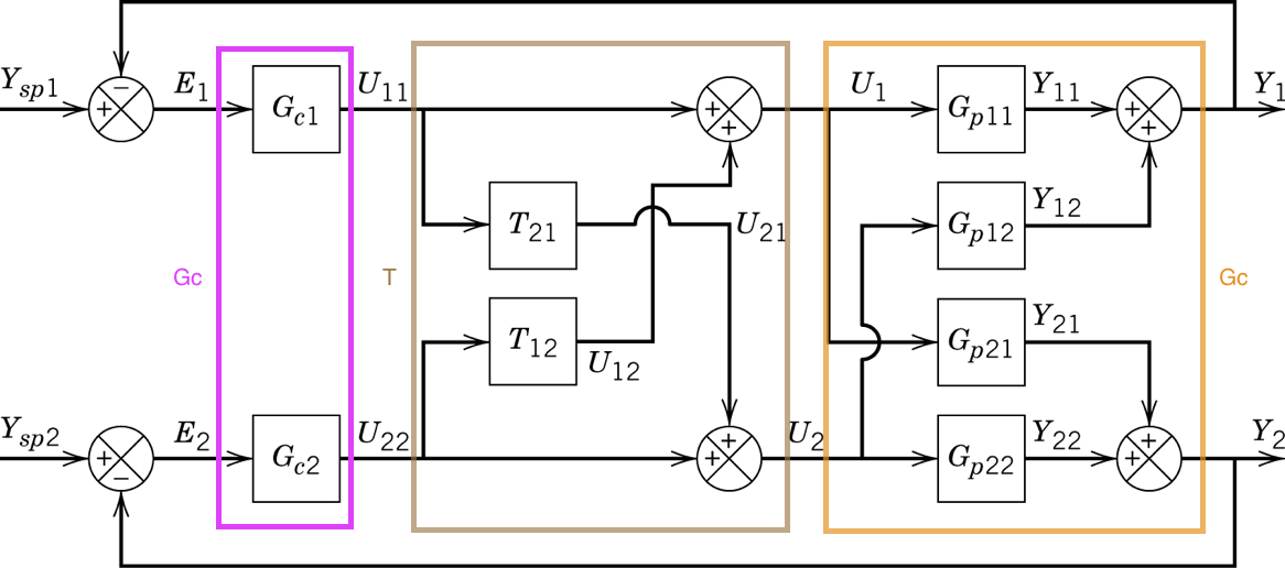
5.2. 2. Zero off-diagonals

A more common strategy is to solve directly for the off-diagonal elements of set equal to zero.

So we just want

\[\begin{split}G_P T = \begin{bmatrix}d_1&0\\0&d_2\end{bmatrix}\end{split}\]

Note the difference between the first method and this one - here we are not specifying the diagonal at all, we just want the off-diagonals to be zero.

T21, T12 = sympy.symbols('T21, T12')
T = sympy.Matrix([[1, T12],
                  [T21, 1]])

wantdiagonal = G_p*T

sol = sympy.solve([wantdiagonal[0,1], wantdiagonal[1, 0]], [T21, T12])

T.subs(sol)

$$\left[\begin{matrix}1 & - \frac{G_{p12}}{G_{p11}}\\- \frac{G_{p21}}{G_{p22}} & 1\end{matrix}\right]$$

So this is the classic/traditional decoupler shown in the diagram (with unit passthrough on the diagonals). This changes the transfer function the controller “sees” to

G_p*T.subs(sol)

$$\left[\begin{matrix}G_{p11} - \frac{G_{p12} G_{p21}}{G_{p22}} & 0\\0 & G_{p22} - \frac{G_{p12} G_{p21}}{G_{p11}}\end{matrix}\right]$$

Pros:

• Relatively simple design process

• Less complicated decoupler than the inverse-based method

Cons:

• Apparent plant may be higher order than the actual plant

• Still requires an inverse, may not be physically realisable (but more likely than method 1)

5.3. 3. Adjugate method

The adjugate (previously calld the adjoint) of a matrix will also diagonalise a system

T = G_p.adjugate()
T

$$\left[\begin{matrix}G_{p22} & - G_{p12}\\- G_{p21} & G_{p11}\end{matrix}\right]$$

G_p*T

$$\left[\begin{matrix}G_{p11} G_{p22} - G_{p12} G_{p21} & 0\\0 & G_{p11} G_{p22} - G_{p12} G_{p21}\end{matrix}\right]$$

Pros:

• Decoupler guaranteed to be physically realisable because it only requires “forward” models of the system.

Cons:

• Apparent plant now much higher order (look at the products in the \(G_pT\) expression)