9. Blocksim
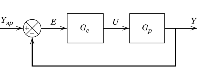
tbcontrol.blocksim is a simple library for simulating the kinds of block diagrams you would encounter in a typical undergraduate control textbook. Let’s start with the most basic example of feedback control.
[1]:
import tbcontrol
tbcontrol.expectversion("0.1.1")
[2]:
from tbcontrol import blocksim
Our first job is to define objects representing each of the blocks. A common one is the LTI block
[3]:
Gp = blocksim.LTI('Gp', 'u', 'y', 10, [100, 1], 50)
[4]:
Gp
[4]:
LTI: u →[ Gp ]→ y
We’ll use a PI controller
[5]:
Gc = blocksim.PI('Gc', 'e', 'u', 0.1, 50)
[6]:
Gc
[6]:
PI: e →[ Gc ]→ u
Once we have the blocks, we can create a Diagram.
Sums are specified as a dictionary with the keys being the output signal and the values being a tuple containing the input signals. The leading + is compulsory.
The inputs come next and are specified as functions of time. Blocksim.step() can be used to build a step function.
[7]:
diagram = blocksim.Diagram([Gp, Gc],
                           sums={'e': ('+ysp', '-y')},
                           inputs={'ysp': blocksim.step()})
[8]:
diagram
[8]:
LTI: u →[ Gp ]→ y
PI: e →[ Gc ]→ u
Blocksim is primarily focused on being able to simulate a diagram. The next step is to create a time vector and do the simulation.
[9]:
import numpy
The time vector also specifies the step size for integration. Since blocksim uses Euler integration internally you should choose a time step which is at least 10 times smaller than the smallest time constant of all the blocks. The timespan is of course dependent on what you are investigating.
[10]:
ts = numpy.arange(start=0, stop=1000, step=1)
[11]:
simulation_results = diagram.simulate(ts, progress=True)
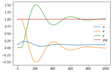
The result of simulate() is a dictionary containing the simulation results.
[12]:
import matplotlib.pyplot as plt
[13]:
%matplotlib inline
[14]:
for signal, value in simulation_results.items():
    plt.plot(ts, value, label=signal)
plt.legend()
[14]:
<matplotlib.legend.Legend at 0x1c19f872b0>
9.1. Re-using parts of a diagram
Let’s compare the output of a PI and a PID controller on this system. We’ve already got the PI response, which we should store.
[15]:
y_pi = simulation_results['y']
Let’s swap out the PI controller for a PID.
[16]:
Gc_pid = blocksim.PID('Gc', 'e', 'u', 0.1, 50, 25)
[17]:
diagram.blocks = [Gp, Gc_pid]
[18]:
simulation_results = diagram.simulate(ts, progress=True)
[19]:
plt.plot(ts, y_pi, label='PI')
plt.plot(ts, simulation_results['y'], label='PID')
plt.legend()
[19]:
<matplotlib.legend.Legend at 0x1c1a113d68>
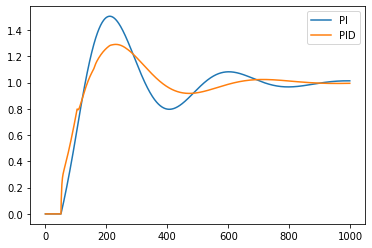
We can see that adding the derivative action has improved control.
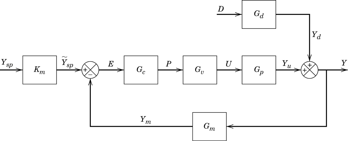
10. Disturbances
We can simulate a more complicated block diagram with a disturbance.
[20]:
Km = blocksim.LTI('Km', 'ysp', 'ytildesp', 1, 1)
Gc = blocksim.PI('Gp', 'e', 'p', Kc=8, tau_i=10)
Gv = blocksim.LTI('Gv', 'p', 'u', 1, 1)
Gp = blocksim.LTI('Gp', 'u', 'yu', [1], [10, 1])
Gd = blocksim.LTI('Gd', 'd', 'yd', [1], [10, 1])
Gm = blocksim.LTI('Gm', 'y', 'ym', [1], [1, 1])

blocks = [Km, Gc, Gv, Gp, Gd, Gm]
[21]:
sums = {'e': ('+ytildesp', '-ym'),
        'y': ('+yd', '+yu')}

inputs = {'ysp': blocksim.step(),
          'd': blocksim.step(starttime=50)}
[22]:
diagram = blocksim.Diagram(blocks, sums, inputs)
[23]:
ts = numpy.arange(start=0, stop=100, step=0.05)
[24]:
results = diagram.simulate(ts, progress=True)
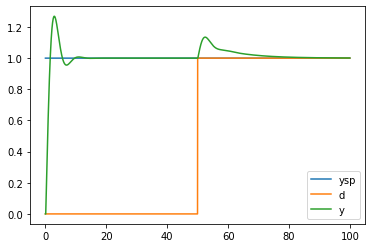
[25]:
for name in ('ysp', 'd', 'y'):
    plt.plot(ts, results[name], label=name)
plt.legend()
[25]:
<matplotlib.legend.Legend at 0x1c19feccf8>
11. Algebraic equations
Sometimes it is useful to be able to handle non-linear calculations in block diagrams. This deviates from the strict interpretation of block diagrams but can be useful for instance in calculating the response of a controller with output limits.
[26]:
import numpy
[27]:
def limit(t, u):
    return numpy.clip(u, 0, 0.2)
[28]:
Gp = blocksim.LTI('Gp', 'ulimited', 'y', 10, [100, 1], 50)
Gc = blocksim.PI('Gc', 'e', 'u', 0.1, 50)
[29]:
limiter = blocksim.AlgebraicEquation('Limiter', 'u', 'ulimited', limit)
[30]:
diagram = blocksim.Diagram([Gp, Gc, limiter],
                           sums={'e': ('+ysp', '-y')},
                           inputs={'ysp': blocksim.step()})
[31]:
ts = numpy.arange(start=0, stop=1000, step=1)
[32]:
simulation_results = diagram.simulate(ts)
[33]:
diagram
[33]:
LTI: ulimited →[ Gp ]→ y
PI: e →[ Gc ]→ u
AlgebraicEquation: u →[ Limiter ]→ ulimited
[34]:
plt.plot(ts, simulation_results['u'])
plt.plot(ts, simulation_results['ulimited'])
[34]:
[<matplotlib.lines.Line2D at 0x1c1a16ad68>]
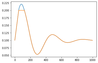
We can see the effect of the limiter clearly in the above figure
[ ]: