83. Multivariable Stability analysis¶

When we used proportional control on SISO systems we observed that there is usually an upper bound on the controller gain $K_c$ above which the controlled system becomes unstable. Let’s investigate the equivalent calculation for MIMO systems.

[1]:

import sympy
sympy.init_printing()
%matplotlib inline

[2]:

s = sympy.Symbol('s')

This matrix is from example 16.2 in Seborg

[3]:

Gp = sympy.Matrix([[2/(10*s + 1), sympy.Rational('1.5')/(s + 1)],
                   [sympy.Rational('1.5')/(s + 1), 2/(10*s + 1)]])
Gp

[3]:

$$\left[\begin{matrix}\frac{2}{10 s + 1} & \frac{3}{2 \left(s + 1\right)}\\\frac{3}{2 \left(s + 1\right)} & \frac{2}{10 s + 1}\end{matrix}\right]$$

[4]:

K_c1, K_c2 = sympy.symbols('K_c1, K_c2', real=True)

Unlike in SISO systems, we now have a choice of pairing. We will see that there are differences in the stability behaviour for the different pairings.

[5]:

diagonal = True

[6]:

if diagonal:
    Gc = sympy.Matrix([[K_c1, 0],
                       [0, K_c2]])
else:
    Gc = sympy.Matrix([[0, K_c2],
                       [K_c1, 0]])

[7]:

I = sympy.Matrix([[1, 0],
                  [0, 1]])

The characteristic equation can be obtained from the $|I + GpGc|$. I divide by 4 here to obtain a final constant of 1 like in the example to make comparison easier. Make sure you understand that any constant multiple of the characteristic equation will have the same poles and zeros.

[8]:

charpoly = sympy.poly(sympy.numer((I + Gp*Gc).det().cancel())/4, s)

Compare with Equation 16-20:

[9]:

charpoly2 = sympy.poly(
    sympy.numer(
        ((1 + Gc[0,0]*Gp[0,0])*(1 + Gc[1,1]*Gp[1,1]) - Gc[0,0]*Gc[1,1]*Gp[0,1]*Gp[1,0]).cancel()
    )/4, s)

[10]:

charpoly == charpoly2

[10]:

True

Now that we have a characteristic polynomial, we can determine stability criteria using the routh function from tbcontrol.symbolic.

[11]:

from tbcontrol.symbolic import routh

[12]:

R = routh(charpoly)

[13]:

R[0, 0]

[13]:

$$100$$

All the remaining elements of the left hand row must be positive (the same sign as the first element)

[14]:

requirements = True
for r in R[1:, 0]:
    requirements = sympy.And(requirements, r>0)

The graph below is supposed to match the textbook, but as of 2019-03-30 it does not. This appears to be a bug in plot_implicit.

[15]:

sympy.plot_implicit(requirements, (K_c2, -2, 7), (K_c1, -2, 4))

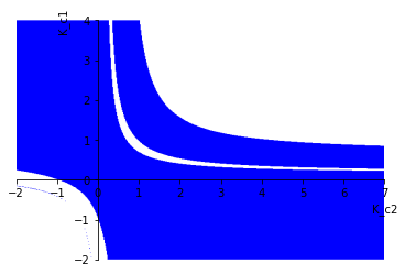
../../_images/2_Control_7_Multivariable_control_Multivariable_stability_analysis_23_0.png

[15]:

<sympy.plotting.plot.Plot at 0x1217574e0>

As an alternative, let’s evaluate numerically

[16]:

import numpy

[17]:

import matplotlib.pyplot as plt
%matplotlib inline

[18]:

f = sympy.lambdify((K_c2, K_c1), requirements)

[19]:

nK_c2, nK_c1 = numpy.meshgrid(numpy.linspace(-2, 4, 300), numpy.linspace(-2, 7, 300))

[20]:

r = f(nK_c2, nK_c1)

[21]:

plt.pcolor(nK_c2, nK_c1, r)
plt.ylabel('K_c1')
plt.xlabel('K_c2')

[21]:

Text(0.5, 0, 'K_c2')

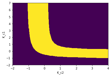
../../_images/2_Control_7_Multivariable_control_Multivariable_stability_analysis_30_1.png

We can see that even this simple system can exhibit more complicated behaviour than we may expect from first order systems because of the extra loops formed by the controllers.