import pandas
import numpy
import matplotlib.pyplot as plt
%matplotlib inline

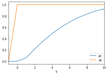
We will fit an ARX model of this form to a step response.

\[y(k) = a_1 y(k - 1) + a_2 y(k - 2) + b_1 u(k - 1) + b_2 u(k - 2)\]

data = pandas.read_csv('../../assets/data.csv', index_col='k')
data['uk'] = 1
data.loc[0] = [0, 1]  # input changes at t=0
data.loc[-1] = [0, 0]  # everything was steady at t < 0
data = data.sort_index()
data

	yk	uk
k
-1	0.000	0
0	0.000	1
1	0.058	1
2	0.217	1
3	0.360	1
4	0.488	1
5	0.600	1
6	0.692	1
7	0.772	1
8	0.833	1
9	0.888	1
10	0.925	1

y = data.yk
u = data.uk

data.plot()

<matplotlib.axes._subplots.AxesSubplot at 0x6215bf828>

We effectively have the following equations (I repeat the equation here for convenience):

\[y(k) = a_1 y(k - 1) + a_2 y(k - 2) + b_1 u(k - 1) + b_2 u(k - 2)\]

for k in range(1, 11):
    print(f'{y[k]:.2} = a1×{y[k - 1]:.2} + a2×{y[k - 2]:.2} + b1×{u[k - 1]} + b2×{u[k - 2]}')

0.058 = a1×0.0 + a2×0.0 + b1×1 + b2×0
0.22 = a1×0.058 + a2×0.0 + b1×1 + b2×1
0.36 = a1×0.22 + a2×0.058 + b1×1 + b2×1
0.49 = a1×0.36 + a2×0.22 + b1×1 + b2×1
0.6 = a1×0.49 + a2×0.36 + b1×1 + b2×1
0.69 = a1×0.6 + a2×0.49 + b1×1 + b2×1
0.77 = a1×0.69 + a2×0.6 + b1×1 + b2×1
0.83 = a1×0.77 + a2×0.69 + b1×1 + b2×1
0.89 = a1×0.83 + a2×0.77 + b1×1 + b2×1
0.93 = a1×0.89 + a2×0.83 + b1×1 + b2×1

pandas.DataFrame([(k,
                  y[k],
                  y[k-1],
                  y[k-2],
                  u[k-1],
                  u[k-2]) for k in range(1, 11)], columns=['k', 'y[k]', 'y[k-1]', 'y[k-2]', 'u[k-1]', 'u[k-2]'])

	k	y[k]	y[k-1]	y[k-2]	u[k-1]	u[k-2]
0	1	0.058	0.000	0.000	1	0
1	2	0.217	0.058	0.000	1	1
2	3	0.360	0.217	0.058	1	1
3	4	0.488	0.360	0.217	1	1
4	5	0.600	0.488	0.360	1	1
5	6	0.692	0.600	0.488	1	1
6	7	0.772	0.692	0.600	1	1
7	8	0.833	0.772	0.692	1	1
8	9	0.888	0.833	0.772	1	1
9	10	0.925	0.888	0.833	1	1

We notice that these equations are linear in the coefficients. We can define \(\beta= [a_1, a_2, b_1, b_2]^T\). Now, to write the above equations in matrix form $Y = X :nbsphinx-math:`beta `$, we define

Y = numpy.atleast_2d(y.loc[1:]).T
Y

array([[0.058],
       [0.217],
       [0.36 ],
       [0.488],
       [0.6  ],
       [0.692],
       [0.772],
       [0.833],
       [0.888],
       [0.925]])

To build the coefficient matrix we observe that there are two blocks of constant diagonals (the part with the \(y\)s and the part with the \(u\)s). Matrices with constant diagonals are called Toeplitz matrices and can be constructed with the scipy.linalg.toeplitz function.

import scipy
import scipy.linalg

X1 = scipy.linalg.toeplitz(y.loc[0:9], [0, 0])
X1

array([[0.   , 0.   ],
       [0.058, 0.   ],
       [0.217, 0.058],
       [0.36 , 0.217],
       [0.488, 0.36 ],
       [0.6  , 0.488],
       [0.692, 0.6  ],
       [0.772, 0.692],
       [0.833, 0.772],
       [0.888, 0.833]])

X2 = scipy.linalg.toeplitz(u.loc[0:9], [0, 0])
X2

array([[1, 0],
       [1, 1],
       [1, 1],
       [1, 1],
       [1, 1],
       [1, 1],
       [1, 1],
       [1, 1],
       [1, 1],
       [1, 1]])

X = numpy.hstack([X1, X2])

X

array([[0.   , 0.   , 1.   , 0.   ],
       [0.058, 0.   , 1.   , 1.   ],
       [0.217, 0.058, 1.   , 1.   ],
       [0.36 , 0.217, 1.   , 1.   ],
       [0.488, 0.36 , 1.   , 1.   ],
       [0.6  , 0.488, 1.   , 1.   ],
       [0.692, 0.6  , 1.   , 1.   ],
       [0.772, 0.692, 1.   , 1.   ],
       [0.833, 0.772, 1.   , 1.   ],
       [0.888, 0.833, 1.   , 1.   ]])

Another option is to use the loop from before to construct the matrices. This is a little more legible but slower:

Y = []
X = []
for k in range(1, 11):
    Y.append([y[k]])
    X.append([y[k - 1], y[k - 2], u[k - 1], u[k - 2]])
Y = numpy.array(Y)
X = numpy.array(X)

We solve for \(\beta\) as we did for linear regression:

beta, _, _, _ = numpy.linalg.lstsq(X, Y, rcond=None)
beta

array([[ 0.98464753],
       [-0.12211256],
       [ 0.058     ],
       [ 0.10124916]])