import sympy
sympy.init_printing()
import matplotlib.pyplot as plt
%matplotlib inline
import tbcontrol
tbcontrol.expectversion('0.1.3')

There is a difference between the \(z\) transform of an impulse response and the equivalent z transform of a continuous system with a hold element.

Let’s consider the system

\[G(s) = \frac{K}{s + r}\]

s, z, q = sympy.symbols('s, z, q')
K, r, t = sympy.symbols('K, r, t', real=True)
Dt = sympy.Symbol(r'\Delta t', positive=True)

G = K/(s + r)

The impulse response of this system is simply the inverse laplace transform:

import tbcontrol.symbolic

gt = sympy.inverse_laplace_transform(G, s, t)
gt

$$K e^{- r t} \theta\left(t\right)$$

The \(z\) transform of this function of time, sampled at a sampling rate of \(\Delta t\) can be read off the table as

b = sympy.exp(-r*Dt)
Gz = K/(1 - b*z**-1)

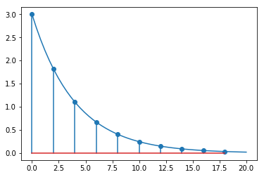
Let’s choose values and plot the response.

parameters = {K: 3, r: 0.25, Dt: 2}

import numpy

ts = numpy.linspace(0, 20)

terms = 10

def plot_discrete(Gz, N, Dt):
    ts = [Dt*n for n in range(N)]
    values = tbcontrol.symbolic.sampledvalues(Gz.subs(parameters), z, N)
    plt.stem(ts, values)

def values(expression, ts):
    return tbcontrol.symbolic.evaluate_at_times(expression.subs(parameters), t, ts)

plt.plot(ts, values(gt, ts))
plot_discrete(Gz, terms, parameters[Dt])

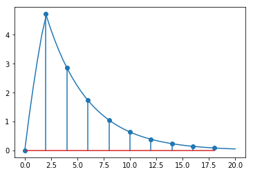
But the value in Table 17.1 is

a1 = -b
b1 = K/r*(1 - b)
Gz_seborg = (b1 * z**-1)/(1 + a1*z**-1)

Gz_seborg

$$\frac{K \left(1 - e^{- \Delta t r}\right)}{r z \left(1 - \frac{e^{- \Delta t r}}{z}\right)}$$

That’s clearly not the same as the discrete transform in the datasheet. What is going on?

The values in the table in seborg are the z transform of the transfer function with a hold element!

The z-transform of this combination can be written \(\mathcal{Z}\{H(s)G(s)\}\). Remember, \(H(s) = \frac{1}{s}(1 - e^{-\Delta t s})\). Now we can show

:nbsphinx-math:`begin{align} mathcal{Z}left{{H(s)G(s)}right} &=

mathcal{Z}left{frac{1}{s}(1 - e^{-Ts})G(s)right} \

&= mathcal{Z}left{underbrace{frac{G(s)}{s}}_{F(s)}(1 - e^{-Ts})right} \

&= mathcal{Z}left{F(s) - F(s)e^{-Ts}right} \

&= mathcal{Z}left{F(s)right} - mathcal{Z}left{F(s)e^{-Ts}right} \ &= F(z) - F(z)z^{-1} \ &= F(z)(1 - z^{-1})

end{align}` So the z transform we’re looking for will be \(F(z)(1 - z^{-1})\) with \(F(z)\) being the transform on the right of the table of \(\frac{1}{s}G(s)\).

To remind ourselves,

G

$$\frac{K}{r + s}$$

So we’re looking for

(G/s)

$$\frac{K}{s \left(r + s\right)}$$

So we should see the same response if we plot this:

There is an element in the table for

\[\frac{a}{s(s + a)}\]

which is the same as what we want but multiplied by \(a\). We should be able to use the associated \(z\) transform:

a = r

table_value = (1 - b)*z**-1/((1 - z**-1)*(1 - b*z**-1))

Fz = K * table_value / a

Fz * (1 - z**-1) == Gz_seborg

True

response = sympy.inverse_laplace_transform(G/s, s, t)

plot_discrete(Gz_seborg, terms, parameters[Dt])
plt.plot(ts, values(response - response.subs(t, t-parameters[Dt]), ts))

[<matplotlib.lines.Line2D at 0x1184bacf8>]